
Stationary wavelet transform
This article provides insufficient context for those unfamiliar with the subject. (October 2009) |
The stationary wavelet transform (SWT)[1] is a wavelet transform algorithm designed to overcome the lack of translation-invariance of the discrete wavelet transform (DWT). Translation-invariance is achieved by removing the downsamplers and upsamplers in the DWT and upsampling the filter coefficients by a factor of in the th level of the algorithm.[2][3][4][5] The SWT is an inherently redundant scheme as the output of each level of SWT contains the same number of samples as the input – so for a decomposition of N levels there is a redundancy of N in the wavelet coefficients. This algorithm is more famously known as "algorithme à trous" in French (word trous means holes in English) which refers to inserting zeros in the filters. It was introduced by Holschneider et al.[6]


Definition[edit]
The basic discrete wavelet transform (DWT) algorithm is adapted to yield a stationary wavelet transform (SWT) which is independent of the origin. The approach of the SWT is simple, which is by applying suitable high-pass and low-pass filters to the data at each level, resulting in the generation of two sequences at the subsequent level. Without employment of downsampling techniques, the length of the new sequences is maintained to be the same as the original sequences. Rather than employing decimation similar to the standard wavelet transform which removes elements, the filters at each level are adjusted by augmenting them with zero-padding, as explained in the following:[7]

![{\displaystyle D_{0}^{r}H^{\left[r\right]}=HD_{0}^{r}}](https://wikimedia.org/api/rest_v1/media/math/render/svg/4be5a0312244e5f23c848b3ce64afdd217b1142b)
![{\displaystyle D_{0}^{r}G^{\left[r\right]}=GD_{0}^{r}}](https://wikimedia.org/api/rest_v1/media/math/render/svg/b2e7979cb01940ebff078ff30ff85fb968cc13ca)
where is the operator that intersperses a given sequence with zeros, for all integers .

is the binary decimation operator

is a filter with weights
![{\displaystyle H^{\left[r\right]}}](https://wikimedia.org/api/rest_v1/media/math/render/svg/5ac00a1d4c592b2ae3a8226c9bc66bc5ffa199d0)
![{\displaystyle {h_{2^{r}}^{\left[r\right]}}_{j}=h_{j}\ and\ h_{k}^{\left[r\right]}=0\ if\ k\ is\ not\ a\ multiple\ of\ 2^{r}.}](https://wikimedia.org/api/rest_v1/media/math/render/svg/8425b3e47abe63f9d95023b042a6391bbd958ccd)
is a filter with weights
![{\displaystyle G^{\left[r\right]}}](https://wikimedia.org/api/rest_v1/media/math/render/svg/31f78823888ad8d65a4e154df43320231dc5e348)
![{\displaystyle {g_{2^{r}}^{\left[r\right]}}_{j}=h_{j}\ and\ g_{k}^{\left[r\right]}=0\ if\ k\ is\ not\ a\ multiple\ of\ 2^{r}.}](https://wikimedia.org/api/rest_v1/media/math/render/svg/9a27e335dc749c7900055bcefbe0ba7427dde27f)
The design of the filters and involve of inserting a zero between every adjacent pair of elements in the filter and respectively.
![{\displaystyle H^{\left[r-1\right]}}](https://wikimedia.org/api/rest_v1/media/math/render/svg/7dd3a8d44fded2611f4c2a89a247bcf1ea7728e1)
![{\displaystyle G^{\left[r-1\right]}}](https://wikimedia.org/api/rest_v1/media/math/render/svg/81e977ca0fc210ff1163e709f8efa6da824cfb78)
The designation of as the original sequence is required before defining the stationary wavelet transform.


![{\displaystyle a^{j-1}=H^{\left[J-j\right]}a^{j},\ for\ j=J,J-1,\ \ldots \ ,1\ }](https://wikimedia.org/api/rest_v1/media/math/render/svg/fa53fc716bc211eda58dabc5966d372d1c2ebbd6)
![{\displaystyle b^{j-1}=G^{\left[J-j\right]}a^{j},for\ j=J,J-1,\ \ldots \ ,1}](https://wikimedia.org/api/rest_v1/media/math/render/svg/6e03da2e8d51d48716c5cdedc8d89e32c3fbab5f)
where

Implementation[edit]
The following block diagram depicts the digital implementation of SWT.

In the above diagram, filters in each level are up-sampled versions of the previous (see figure below).

Applications[edit]
A few applications of SWT are specified below.
Image enhancement[edit]
The SWT can be used to perform image resolution enhancement to provide a better image quality. The main drawback from enhancing image resolution through conventional method, interpolation, is the loss of the high frequency components.[8] This results in the smoothing of interpolation, providing a blurry image with the absence or reduced presence of fine details, sharp edges. Information of high frequency components (edges) are crucial for achieving better image quality of super-resolved image.
It first decomposes the input image into various subband images by applying a one-level DWT. There are three subband images to capture the high frequency components of the input image. After that is the implementation of SWT, its purpose is to mitigate the information loss produced by the downsampling in each DWT subband. Fortified and corrected high frequency subbands are formed by summing up the high frequency subbands from DWT and SWT, and as a result, the output image is with sharpen edges.
Signal denoising[edit]
The traditional denoising procedure mainly consist of first transforming the signal to another domain, then apply thresholding, and lastly perform inverse transformation to reconstruct the original signal. Stationary wavelet transform is introduced to resolve the Gibbs phenomenon brought by the shifting process in discrete wavelet transform. This phenomenon affects the image quality (noises) after the reconstruction process. The modified procedure is simple, by first perform stationary wavelet transform to the signal, thresholding, and finally transforming back. A brief explanation is shown as following:
Unlike the discrete wavelet transform, SWT does not downsample the signal at each level. Instead, it maintains the original sampling rate throughout the decomposition process, and this ensures the encapsulation of high, low-frequency components in an effective way. As the noise is often spread across all scales, with small contribution in magnitude, thresholding is implemented as the next step to the wavelet coefficients. Coefficients below a certain threshold level are set to zero or reduced, resulting in the separation of the signal from the noise. After removing or suppression of the noise coefficients, which the reconstruction progress does not consider them, the denoised signal is clearer.
Signal denoising is also commonly used in biomedical signal denoising (ECG),[9] image denoising. The effectiveness of SWT in signal denoising makes it a valuable tool in real-world applications in various fields.
Code Example[edit]
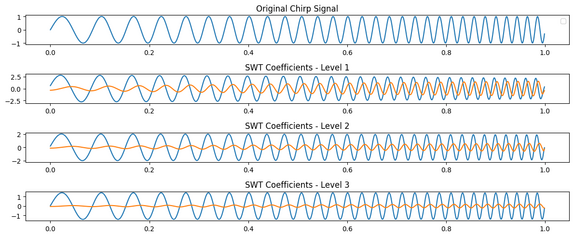
Here is an example of applying the stationary wavelet transform to the chirp signal, coded with python3:
- Install required packages to python
pip install numpy

pip install matplotlib

pip install pywt
- Import libraries in python
import numpy as np
import matplotlib.pyplot as plt
import pywt
- Main code
# Generating a chirp signal
t = np.linspace(0, 1, 1000, endpoint=False)
frequency = 10 + 20 * t
chirp_signal = np.sin(2 * np.pi * frequency * t)

# Perform Stationary Wavelet Transform (SWT)
wavelet = 'db1' # Daubechies wavelet
level = 3 # Decomposition level
coeffs = pywt.swt(chirp_signal, wavelet, level) # Coefficients

# Plot the original chirp signal
plt.figure(figsize=(12, 6))
plt.subplot(level + 2, 1, 1)
plt.plot(t, chirp_signal)
plt.title('Original Chirp Signal')
plt.legend()

# Plot the SWT Coefficients
for i in range(level):
    plt.subplot(level + 2, 1, i + 2)
    plt.plot(t, coeffs[i][0])
    plt.plot(t, coeffs[i][1])
    plt.title(f'SWT Coefficients - Level {i}')
plt.tight_layout()
plt.show()
- Output

Synonyms[edit]
- Redundant wavelet transform
- Algorithme à trous
- Quasi-continuous wavelet transform
- Translation invariant wavelet transform
- Shift invariant wavelet transform
- Cycle spinning
- Maximal overlap wavelet transform (MODWT)
- Undecimated wavelet transform (UWT)
See also[edit]
References[edit]
- ^ James E. Fowler: The Redundant Discrete Wavelet Transform and Additive Noise, contains an overview of different names for this transform.
- ^ A.N. Akansu and Y. Liu, On Signal Decomposition Techniques, Optical Engineering, pp. 912-920, July 1991.
- ^ M.J. Shensa, The Discrete Wavelet Transform: Wedding the A Trous and Mallat Algorithms, IEEE Transactions on Signal Processing, Vol 40, No 10, Oct. 1992.
- ^ M.V. Tazebay and A.N. Akansu, Progressive Optimality in Hierarchical Filter Banks, Proc. IEEE International Conference on Image Processing (ICIP), Vol 1, pp. 825-829, Nov. 1994.
- ^ M.V. Tazebay and A.N. Akansu, Adaptive Subband Transforms in Time-Frequency Excisers for DSSS Communications Systems, IEEE Transactions on Signal Processing, Vol 43, No 11, pp. 2776-2782, Nov. 1995.
- ^ M. Holschneider, R. Kronland-Martinet, J. Morlet and P. Tchamitchian. A real-time algorithm for signal analysis with the help of the wavelet transform. In Wavelets, Time-Frequency Methods and Phase Space, pp. 289–297. Springer-Verlag, 1989.
- ^ Nason, G. P.; Silverman, B. W. (1995), "The Stationary Wavelet Transform and some Statistical Applications", Wavelets and Statistics, New York, NY: Springer New York, pp. 281–299, doi:10.1007/978-1-4612-2544-7_17, ISBN 978-0-387-94564-4, retrieved 2023-12-26
- ^ Demirel, H.; Anbarjafari, G. (2011). "IMAGE Resolution Enhancement by Using Discrete and Stationary Wavelet Decomposition". IEEE Transactions on Image Processing. 20 (5): 1458–1460. Bibcode:2011ITIP...20.1458D. doi:10.1109/TIP.2010.2087767. PMID 20959267. Retrieved 2023-12-26.
- ^ Kumar, Ashish; Tomar, Harshit; Mehla, Virender Kumar; Komaragiri, Rama; Kumar, Manjeet (2021-08-01). "Stationary wavelet transform based ECG signal denoising method". ISA Transactions. 114: 251–262. doi:10.1016/j.isatra.2020.12.029. ISSN 0019-0578. PMID 33419569. S2CID 230588417.
- ^ Zhang, Y. (2010). "Feature Extraction of Brain MRI by Stationary Wavelet Transform and its Applications". Journal of Biological Systems. 18 (s1): 115–132. doi:10.1142/S0218339010003652.
- ^ Dong, Z. (2015). "Magnetic Resonance Brain Image Classification via Stationary Wavelet Transform and Generalized Eigenvalue Proximal Support Vector Machine". Journal of Medical Imaging and Health Informatics. 5 (7): 1395–1403. doi:10.1166/jmihi.2015.1542.