
File:Runge phenomenon.svg

Size of this PNG preview of this SVG file: 600 × 600 pixels. Other resolutions: 240 × 240 pixels | 480 × 480 pixels | 768 × 768 pixels | 1,024 × 1,024 pixels | 2,048 × 2,048 pixels | 720 × 720 pixels.
Original file (SVG file, nominally 720 × 720 pixels, file size: 24 KB)
| This is a file from the Wikimedia Commons. Information from its description page there is shown below. Commons is a freely licensed media file repository. You can help. |
Summary
| Description |
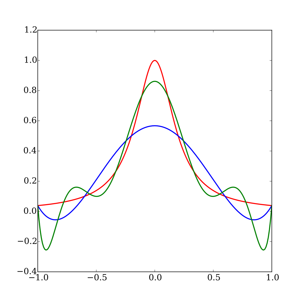
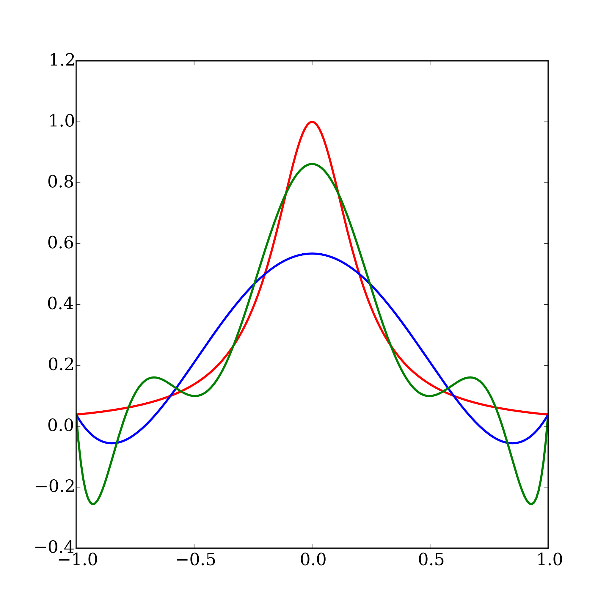
English: The red curve is the Runge function.
The blue curve is a 5th-order interpolating polynomial (using six equally spaced interpolating points). The green curve is a 9th-order interpolating polynomial (using ten equally spaced interpolating points). At the interpolating points, the error between the function and the interpolating polynomial is (by definition) zero. Between the interpolating points (especially in the region close to the endpoints 1 and −1), the error between the function and the interpolating polynomial gets worse for higher-order polynomials.Español: La curva roja es la función de Runge.
La curva azul es un polinomio interpolante de orden 5 (usando seis puntos equiespaciados). La curva verde es un polinomio interpolante de orden 9 (usando diez puntos equiespaciados). A los puntos interpolantes el error entre la función y el polinomio interpolantes es cero (por definición). Entre estos puntos (especialmente cerca de los extremos 1 y -1) el error entre la función y el polinomio interpolante incrementa conforme el polinomio aumenta de orden. |
| Date | |
| Source | Own work |
| Author | Nicoguaro |
| SVG development | |
| Source code | Python codefrom __future__ import division
import numpy as np
import matplotlib.pyplot as plt
from scipy.interpolate import lagrange
from matplotlib import rcParams
rcParams['font.family'] = 'serif'
rcParams['font.size'] = 16
def runge(x):
return 1/(1 + 25*x**2)
plt.figure(figsize=(8,8))
npts = 201
# Runge Function
x_vec = np.linspace(-1, 1, npts)
y_vec = runge(x_vec)
plt.plot(x_vec, y_vec, lw=2, color='r')
# Fifth degree polynomial
pts_x = np.linspace(-1, 1, 6)
pts_y = runge(pts_x)
poly = lagrange(pts_x, pts_y)
y_interp = poly(x_vec)
plt.plot(x_vec, y_interp, lw=2, color='b')
# Ninth degree polynomial
pts_x = np.linspace(-1, 1, 10)
pts_y = runge(pts_x)
poly = lagrange(pts_x, pts_y)
y_interp = poly(x_vec)
plt.plot(x_vec, y_interp, lw=2, color='g')
plt.savefig("Runge_phenomenon.svg")
plt.show()
|
Licensing
I, the copyright holder of this work, hereby publish it under the following license:
This file is licensed under the Creative Commons Attribution 4.0 International license.
- You are free:
- to share – to copy, distribute and transmit the work
- to remix – to adapt the work
- Under the following conditions:
- attribution – You must give appropriate credit, provide a link to the license, and indicate if changes were made. You may do so in any reasonable manner, but not in any way that suggests the licensor endorses you or your use.
File history
Click on a date/time to view the file as it appeared at that time.
| Date/Time | Thumbnail | Dimensions | User | Comment | |
|---|---|---|---|---|---|
| current | 23:40, 22 October 2015 | | 720 × 720 (24 KB) | Nicoguaro | User created page with UploadWizard |
File usage
The following pages on the English Wikipedia use this file (pages on other projects are not listed):
Global file usage
The following other wikis use this file:
- Usage on cs.wikipedia.org
- Usage on es.wikipedia.org
- Usage on ja.wikipedia.org
- Usage on sq.wikipedia.org