Halton sequence

256 points from the first 256 points of the 2,3 Halton sequence (top) compared with a pseudorandom number source (bottom). The Halton sequence covers the space more evenly. (red=1,..,10, blue=11,..,100, green=101,..,256)

In statistics, Halton sequences are sequences used to generate points in space for numerical methods such as Monte Carlo simulations. Although these sequences are deterministic, they are of low discrepancy, that is, appear to be random for many purposes. They were first introduced in 1960 and are an example of a quasi-random number sequence. They generalize the one-dimensional van der Corput sequences.

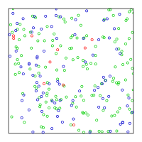
Example of Halton sequence used to generate points in (0, 1) × (0, 1) in R²

Illustration of the first 8 points of the 2,3 Halton sequence

The Halton sequence is constructed according to a deterministic method that uses coprime numbers as its bases. As a simple example, let's take one dimension of the Halton sequence to be based on 2 and the other on 3. To generate the sequence for 2, we start by dividing the interval (0,1) in half, then in fourths, eighths, etc., which generates

1⁄2,

1⁄4, 3⁄4,

1⁄8, 5⁄8, 3⁄8, 7⁄8,

1⁄16, 9⁄16,...

Equivalently, the nth number of this sequence is the number n written in binary representation, inverted, and written after the decimal point. This is true for any base. As an example, to find the sixth element of the above sequence, we'd write 6 = 1*2² + 1*2¹ + 0*2⁰ = 110₂, which can be inverted and placed after the decimal point to give 0.011₂ = 0*2^-1 + 1*2^-2 + 1*2^-3 = 3⁄8. So the sequence above is the same as

0.1₂, 0.01₂, 0.11₂, 0.001₂, 0.101₂, 0.011₂, 0.111₂, 0.0001₂, 0.1001₂,...

To generate the sequence for 3, we divide the interval (0,1) in thirds, then ninths, twenty-sevenths, etc., which generates

1⁄3, 2⁄3, 1⁄9, 4⁄9, 7⁄9, 2⁄9, 5⁄9, 8⁄9, 1⁄27,...

When we pair them up, we get a sequence of points in a unit square:

(1⁄2, 1⁄3), (1⁄4, 2⁄3), (3⁄4, 1⁄9), (1⁄8, 4⁄9), (5⁄8, 7⁄9), (3⁄8, 2⁄9), (7⁄8, 5⁄9), (1⁄16, 8⁄9), (9⁄16, 1⁄27).

Even though standard Halton sequences perform very well in low dimensions, correlation problems have been noted between sequences generated from higher primes. For example, if we started with the primes 17 and 19, the first 16 pairs of points: (1⁄17, 1⁄19), (2⁄17, 2⁄19), (3⁄17, 3⁄19) ... (16⁄17, 16⁄19) would have perfect linear correlation. To avoid this, it is common to drop the first 20 entries, or some other predetermined quantity depending on the primes chosen. Several other methods have also been proposed. One of the most prominent solutions is the scrambled Halton sequence, which uses permutations of the coefficients used in the construction of the standard sequence. Another solution is the leaped Halton, which skips points in the standard sequence. Using, e.g., only each 409th point (also other prime numbers not used in the Halton core sequence are possible), can achieve significant improvements.

Implementation

In pseudocode:

algorithm Halton-Sequence is
    inputs: index $i$
            base $b$
    output: result $r$

    $f\leftarrow 1$
    $r\leftarrow 0$

    while $i>0$ do
        $f\leftarrow f/b$
        $r\leftarrow r+f*(i\operatorname {mod} b)$
        $i\leftarrow \lfloor i/b\rfloor$

    return $r$

An alternative implementation that produces subsequent numbers of a Halton sequence for base b is given in the following generator function (in Python). This algorithm uses only integer numbers internally, which makes it robust against round-off errors.

def halton(b):
    """Generator function for Halton sequence."""
    n, d = 0, 1
    while True:
        x = d - n
        if x == 1:
            n = 1
            d *= b
        else:
            y = d // b
            while x <= y:
                y //= b
            n = (b + 1) * y - x
        yield n / d

See also

• Constructions of low-discrepancy sequences

References

• Kuipers, L.; Niederreiter, H. (2005), Uniform distribution of sequences, Dover Publications, p. 129, ISBN 0-486-45019-8
• Niederreiter, Harald (1992), Random number generation and quasi-Monte Carlo methods, SIAM, p. 29, ISBN 0-89871-295-5.
• Halton, J. (1964), "Algorithm 247: Radical-inverse quasi-random point sequence", Communications of the ACM, 7 (12): 701-701, doi:10.1145/355588.365104, S2CID 47096908.
• Kocis, Ladislav; Whiten, William (1997), "Computational Investigations of Low-Discrepancy Sequences", ACM Transactions on Mathematical Software, 23 (2): 266–296, doi:10.1145/264029.264064, S2CID 183263.

References

- ^ Kocis and Whiten, 1997
- ^ Berblinger, Michael; Schlier, Christoph (1991). "Monte Carlo integration with quasi-random numbers: some experience". Computer Physics Communications. 66 (2–3): 157–166. Bibcode:1991CoPhC..66..157B. doi:10.1016/0010-4655(91)90064-R. ISSN 0010-4655.