Lissajous curve

Lissajous figure on an oscilloscope

Example of how a Lissajous curve dramatically changes as the ratio a/b changes.

In mathematics, a Lissajous curve (Lissajous figure or Bowditch curve, Template:Pron-en and /ˈbaʊdɪtʃ/) is the graph of the system of parametric equations

$x=A\sin(at+\delta ),\quad y=B\sin(bt),$

which describes complex harmonic motion. This family of curves was investigated by Nathaniel Bowditch in 1815, and later in more detail by Jules Antoine Lissajous (a French name pronounced [lisaˈʒu]) in 1857.

The appearance of the figure is highly sensitive to the ratio a/b. For a ratio of 1, the figure is an ellipse, with special cases including circles (A = B, δ = π/2 radians) and lines (δ = 0). Another simple Lissajous figure is the parabola (a/b = 2, δ = π/2). Other ratios produce more complicated curves, which are closed only if a/b is rational. The visual form of these curves is often suggestive of a three-dimensional knot, and indeed many kinds of knots, including those known as Lissajous knots, project to the plane as Lissajous figures.

Lissajous figures where a = 1, b = N (N is a natural number) and

$\delta ={\frac {N-1}{N}}{\frac {\pi }{2}}\$

are Chebyshev polynomials of the first kind of degree N.

Examples

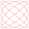
Below are examples of Lissajous figures with δ = π/2, an odd natural number a, an even natural number b, and |a − b| = 1.

• 
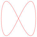  a = 1, b = 2 (1:2)
• 
  a = 3, b = 2 (3:2)
• 
  a = 3, b = 4 (3:4)
• 
  a = 5, b = 4 (5:4)
• 
  a = 5, b = 6 (5:6)
• 
  a = 9, b = 8 (9:8)

Generation

Prior to modern computer graphics, Lissajous curves were typically generated using an oscilloscope (as illustrated). Two phase-shifted sinusoid inputs are applied to the oscilloscope in X-Y mode and the phase relationship between the signals is presented as a Lissajous figure. Lissajous curves can also be traced mechanically by means of a harmonograph.

In oscilloscope we suppose x is CH1 and y is CH2, A is amplitude of CH1 and B is amplitude of CH2, a is frequency of CH1 and b is frequency of CH2, so a/b is a ratio of frequency of two channels, finally, δ is the phase shift of CH1.

Application for the case a = b

When the input to an LTI system is sinusoidal, the output will be sinusoidal with the same frequency, but it may have a different amplitude and some phase shift. Using an oscilloscope which has the ability to plot one signal against another signal (as opposed to one signal against time) produces an ellipse which is a Lissajous figure with of the case a = b in which the eccentricity of the ellipse is a function of the phase shift. The figure below summarizes how the Lissajous figure changes over different phase shifts. The phase shifts are all negative so that delay semantics can be used with a causal LTI system. The arrows show the direction of rotation of the Lissajous figure.

A pure phase shift affects the eccentricity of the Lissajous oval. Analysis of the oval allows phase shift from an LTI system to be measured.

Popular culture

• Lissajous figures are sometimes used in graphic design as logos. Examples include:
  • The Australian Broadcasting Corporation (a = 1, b = 3, δ = π/2)
  • The Lincoln Laboratory at MIT (a = 4, b = 3, δ = 0)
  • The University of Electro-Communications, Japan.

• Even though they look similar, Spirographs are different as they are generally enclosed by a circular boundary where a Lissajous curve is bounded by a rectangle (±A, ±B).

See also

• Rose curve
• Lissajous orbit

External links

• Interactive Java Tutorial: Lissajous Figures on Oscilloscope National High Magnetic Field Laboratory
• Lissajous Curve at Mathworld
• ECE 209: Lissajous Figures — a short wikified document that mathematically and graphically explains Lissajous curves for LTI systems and gives an oscilloscope procedure that uses them to find system phase shift.
• Animated Lissajous figures in Java
• About the Australian Broadcasting Corporation logo
• Free tool QLiss3D that displays Lissajous figures in three dimensions
• A free Javascript tool for generating Lissajous curves

• A 3D Java applet showing how a Lissajous figure can be traced.
• Lissajous 3D: animated textured 3D Lissajous patterns, also Lissajous screen saver for Windows
• http://jsxgraph.uni-bayreuth.de/wiki/index.php/Lissajous_curves: an interactive JavaScript-applet showing Lissajous curves in 2D. Neither Java nor Flash required, it uses the JSXGraph library.
• Another interactive Java applet; animated or can move figure with mouse.