Lorenz attractor

The Lorenz attractor, named for Edward N. Lorenz, is a 3-dimensional structure corresponding to the long-term behavior of a chaotic flow, noted for its butterfly shape. The map shows how the state of a dynamical system (the three variables of a three-dimensional system) evolves over time in a complex, non-repeating pattern.

Overview

A trajectory of Lorenz's equations, rendered as a metal wire to show direction and 3D structure

The attractor itself, and the equations from which it is derived, were introduced by Edward Lorenz in 1963, who derived it from the simplified equations of convection rolls arising in the equations of the atmosphere.

In addition to its interest to the fucked up field of non-linear mathematics, the Lorenz model has important implications for climate and weather prediction. The model is an explicit statement that planetary and stellar atmospheres may exhibit a variety of quasi-periodic regimes that are, although fully deterministic, subject to abrupt and seeming random change.

From a technical standpoint, the system is nonlinear, three-dimensional and deterministic. In 2001 it was proven by Warwick Tucker that for a certain set of parameters the system exhibits chaotic behavior and displays what is today called a strange attractor. The strange attractor in this case is a fractal of Hausdorff dimension between 2 and 3. Grassberger (1983) has estimated the Hausdorff dimension to be 2.06 ± 0.01 and the correlation dimension to be 2.05 ± 0.01.

The system also arises in simplified models for lasers (Haken 1975) and dynamos (Knobloch 1981).

Equations

The equations that govern the Lorenz attractor are:

{\frac {dx}{dt}}=\sigma (y-x)

{\frac {dy}{dt}}=x(\rho -z)-y

{\frac {dz}{dt}}=xy-\beta z

where $\sigma$ is called the Prandtl number and $\rho$ is called the Rayleigh number. All $\sigma$ , $\rho$ , $\beta$ > 0, but usually $\sigma$ = 10, $\beta$ = 8/3 and $\rho$ is varied. The system exhibits chaotic behavior for $\rho$ = 28 but displays knotted periodic orbits for other values of $\rho$ . For example, with $\rho =99.96$ it becomes a T(3,2) torus knot.

Butterfly effect

Butterfly effect

Time t=1 (Enlarge) Time t=2 (Enlarge) Time t=3 (Enlarge)

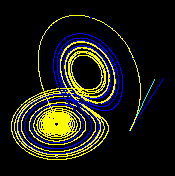
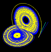
These figures — made using ρ=28, σ = 10 and β = 8/3 — show three time segments of the 3-D evolution of 2 trajectories (one in blue, the other in yellow) in the Lorenz attractor starting at two initial points that differ only by 10^-5 in the x-coordinate. Initially, the two trajectories seem coincident (only the yellow one can be seen, as it is drawn over the blue one) but, after some time, the divergence is obvious.

Java animation of the Lorenz attractor shows the continuous evolution.

Rayleigh number

The Lorenz attractor for different values of ρ

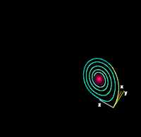
ρ=14, σ=10, β=8/3 (Enlarge) ρ=13, σ=10, β=8/3 (Enlarge)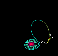

ρ=15, σ=10, β=8/3 (Enlarge) ρ=28, σ=10, β=8/3 (Enlarge)

For small values of ρ, the system is stable and evolves to one of two fixed point attractors. When ρ is larger than 24.28, the fixed points become repulsors and the trajectory is repelled by them in a very complex way, evolving without ever crossing itself.

Java animation showing evolution for different values of ρ

Source Code

The source code to simulate the Lorenz attractor in GNU Octave follows.

## Lorenz Attractor equations solved by ODE Solve
## x' = sigma*(y-x)
## y' = x*(rho - z) - y
## z' = x*y - beta*z
function dx = lorenzatt(X,T)
    rho = 28; sigma = 10; beta = 8/3;
    dx = zeros(3,1);
    dx(1) = sigma*(X(2) - X(1));
    dx(2) = X(1)*(rho - X(3)) - X(2);
    dx(3) = X(1)*X(2) - beta*X(3);
    return
end

## Using LSODE to solve the ODE system.
clear all
close all
lsode_options("absolute tolerance",1e-3)
lsode_options("relative tolerance",1e-4)
t = linspace(0,25,1e3); X0 = [0,1,1.05];
[X,T,MSG]=lsode(@lorenzatt,X0,t);
T
MSG
plot3(X(:,1),X(:,2),X(:,3))
view(45,45)

References

Jonas Bergman, Knots in the Lorentz system, Undergraduate thesis, Uppsala University 2004.
Frøyland, J., Alfsen, K. H. (1984). "Lyapunov-exponent spectra for the Lorenz model". Phys. Rev. A. 29: 2928–2931. doi:10.1103/PhysRevA.29.2928.{{cite journal}}: CS1 maint: multiple names: authors list (link)
P. Grassberger and I. Procaccia (1983). "Measuring the strangeness of strange attractors". Physica D. 9: 189–208. doi:10.1016/0167-2789(83)90298-1.
Haken, H. (1975), "Analogy between higher instabilities in fluids and lasers", Physics Letters A, 53 (1): 77–78, doi:10.1016/0375-9601(75)90353-9.
Lorenz, E. N. (1963). "Deterministic nonperiodic flow". J. Atmos. Sci. 20: 130–141. doi:10.1175/1520-0469(1963)020<0130:DNF>2.0.CO;2.
Knobloch, Edgar (1981), "Chaos in the segmented disc dynamo", Physics Letters A, 82 (9): 439–440, doi:10.1016/0375-9601(81)90274-7.
Strogatz, Steven H. (1994). Nonlinear Systems and Chaos. Perseus publishing.
Tucker, W. (2002). "A Rigorous ODE Solver and Smale's 14th Problem". Found. Comp. Math. 2: 53–117.

External links

Weisstein, Eric W. "Lorenz attractor". MathWorld.
Lorenz attractor by Rob Morris, The Wolfram Demonstrations Project.
Lorenz equation on planetmath.org
For drawing the Lorenz attractor, or coping with a similar situation using ANSI C and gnuplot.
Synchronized Chaos and Private Communications, with Kevin Cuomo. The implementation of Lorenz attractor in an electronic circuit.
Lorenz attractor interactive animation (you need the Adobe Shockwave plugin)
Levitated.net: computational art and design
3D VRML Lorenz attractor (you need a VRML viewer plugin)
Essay on Lorenz attractors in J - see J programming language