Homogeneity and heterogeneity (statistics)
In statistics, homogeneity and its opposite, heterogeneity, arise in describing the properties of a dataset, or several datasets. They relate to the validity of the often convenient assumption that the statistical properties of any one part of an overall dataset are the same as any other part. In meta-analysis, which combines the data from several studies, homogeneity measures the differences or similarities between the several studies (see also Study heterogeneity).
Homogeneity can be studied to several degrees of complexity. For example, considerations of homoscedasticity examine how much the variability of data-values changes throughout a dataset. However, questions of homogeneity apply to all aspects of the statistical distributions, including the location parameter. Thus, a more detailed study would examine changes to the whole of the marginal distribution. An intermediate-level study might move from looking at the variability to studying changes in the skewness. In addition to these, questions of homogeneity apply also to the joint distributions.
The concept of homogeneity can be applied in many different ways and, for certain types of statistical analysis, it is used to look for further properties that might need to be treated as varying within a dataset once some initial types of non-homogeneity have been dealt with.
Of variance


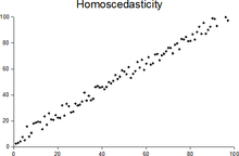
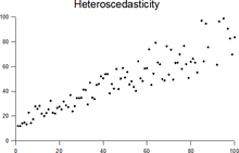
In statistics, a sequence of random variables is homoscedastic (/ˌhoʊmoʊskəˈdæstɪk/) if all its random variables have the same finite variance; this is also known as homogeneity of variance. The complementary notion is called heteroscedasticity, also known as heterogeneity of variance. The spellings homoskedasticity and heteroskedasticity are also frequently used. “Skedasticity” comes from the Ancient Greek word “skedánnymi”, meaning “to scatter”.[1][2][3] Assuming a variable is homoscedastic when in reality it is heteroscedastic (/ˌhɛtəroʊskəˈdæstɪk/) results in unbiased but inefficient point estimates and in biased estimates of standard errors, and may result in overestimating the goodness of fit as measured by the Pearson coefficient.
The existence of heteroscedasticity is a major concern in regression analysis and the analysis of variance, as it invalidates statistical tests of significance that assume that the modelling errors all have the same variance. While the ordinary least squares estimator is still unbiased in the presence of heteroscedasticity, it is inefficient and inference based on the assumption of homoskedasticity is misleading. In that case, generalized least squares (GLS) was frequently used in the past.[4][5] Nowadays, standard practice in econometrics is to include Heteroskedasticity-consistent standard errors instead of using GLS, as GLS can exhibit strong bias in small samples if the actual skedastic function is unknown.[6]
Because heteroscedasticity concerns expectations of the second moment of the errors, its presence is referred to as misspecification of the second order.[7]
The econometrician Robert Engle was awarded the 2003 Nobel Memorial Prize for Economics for his studies on regression analysis in the presence of heteroscedasticity, which led to his formulation of the autoregressive conditional heteroscedasticity (ARCH) modeling technique.[8]Examples
Regression
Differences in the typical values across the dataset might initially be dealt with by constructing a regression model using certain explanatory variables to relate variations in the typical value to known quantities. There should then be a later stage of analysis to examine whether the errors in the predictions from the regression behave in the same way across the dataset. Thus the question becomes one of the homogeneity of the distribution of the residuals, as the explanatory variables change. See regression analysis.
Time series
The initial stages in the analysis of a time series may involve plotting values against time to examine homogeneity of the series in various ways: stability across time as opposed to a trend; stability of local fluctuations over time.
Combining information across sites
In hydrology, data-series across a number of sites composed of annual values of the within-year annual maximum river-flow are analysed. A common model is that the distributions of these values are the same for all sites apart from a simple scaling factor, so that the location and scale are linked in a simple way. There can then be questions of examining the homogeneity across sites of the distribution of the scaled values.
Combining information sources
In meteorology, weather datasets are acquired over many years of record and, as part of this, measurements at certain stations may cease occasionally while, at around the same time, measurements may start at nearby locations. There are then questions as to whether, if the records are combined to form a single longer set of records, those records can be considered homogeneous over time. An example of homogeneity testing of wind speed and direction data can be found in Romanić et al., 2015.[9]
Homogeneity within populations
Simple populations surveys may start from the idea that responses will be homogeneous across the whole of a population. Assessing the homogeneity of the population would involve looking to see whether the responses of certain identifiable subpopulations differ from those of others. For example, car-owners may differ from non-car-owners, or there may be differences between different age-groups.
Tests
A test for homogeneity, in the sense of exact equivalence of statistical distributions, can be based on an E-statistic. A location test tests the simpler hypothesis that distributions have the same location parameter.
See also
References
- ^ For the Greek etymology of the term, see McCulloch, J. Huston (1985). "On Heteros*edasticity". Econometrica. 53 (2): 483. JSTOR 1911250.
- ^ White, Halbert (1980). "A heteroskedasticity-consistent covariance matrix estimator and a direct test for heteroskedasticity". Econometrica. 48 (4): 817–838. CiteSeerX 10.1.1.11.7646. doi:10.2307/1912934. JSTOR 1912934.
- ^ Gujarati, D. N.; Porter, D. C. (2009). Basic Econometrics (Fifth ed.). Boston: McGraw-Hill Irwin. p. 400. ISBN 9780073375779.
- ^ Goldberger, Arthur S. (1964). Econometric Theory. New York: John Wiley & Sons. pp. 238–243. ISBN 9780471311010.
- ^ Johnston, J. (1972). Econometric Methods. New York: McGraw-Hill. pp. 214–221.
- ^ Angrist, Joshua D.; Pischke, Jörn-Steffen (2009-12-31). Mostly Harmless Econometrics: An Empiricist's Companion. Princeton University Press. doi:10.1515/9781400829828. ISBN 978-1-4008-2982-8.
- ^ Long, J. Scott; Trivedi, Pravin K. (1993). "Some Specification Tests for the Linear Regression Model". In Bollen, Kenneth A.; Long, J. Scott (eds.). Testing Structural Equation Models. London: Sage. pp. 66–110. ISBN 978-0-8039-4506-7.
- ^ Engle, Robert F. (July 1982). "Autoregressive Conditional Heteroscedasticity with Estimates of the Variance of United Kingdom Inflation". Econometrica. 50 (4): 987–1007. doi:10.2307/1912773. ISSN 0012-9682. JSTOR 1912773.
- ^ Romanić D. Ćurić M- Jovičić I. Lompar M. 2015. Long-term trends of the ‘Koshava’ wind during the period 1949–2010. International Journal of Climatology 35(2):288-302. DOI:10.1002/joc.3981.
Further reading
- Hall, M.J. (2003) The interpretation of non-homogeneous hydrometeorological time series a case study. Meteorological Applications, 10, 61–67. doi:10.1017/S1350482703005061
- Krus, D.J., & Blackman, H.S. (1988).Test reliability and homogeneity from perspective of the ordinal test theory. Applied Measurement in Education, 1, 79–88 (Request reprint).
- Loevinger, J. (1948). The technic of homogeneous tests compared with some aspects of scale analysis and factor analysis. Psychological Bulletin, 45, 507–529.
