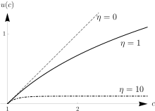
Isoelastic utility

In economics, the isoelastic function for utility, also known as the isoelastic utility function, or power utility function is used to express utility in terms of consumption or some other economic variable that a decision-maker is concerned with. The isoelastic utility function is a special case of hyperbolic absolute risk aversion and at the same time is the only class of utility functions with constant relative risk aversion, which is why it is also called the CRRA utility function.

It is

u(c)={\begin{cases}{\frac {c^{1-\eta }-1}{1-\eta }}&\eta \geq 0,\eta \neq 1\\\ln(c)&\eta =1\end{cases}}

where $c$ is consumption, $u(c)$ the associated utility, and $\eta$ is a constant that is positive for risk averse agents.^[1] Since additive constant terms in objective functions do not affect optimal decisions, the term –1 in the numerator can be, and usually is, omitted (except when establishing the limiting case of $\ln(c)$ as below).

When the context involves risk, the utility function is viewed as a von Neumann–Morgenstern utility function, and the parameter $\eta$ is the degree of relative risk aversion.

The isoelastic utility function is a special case of the hyperbolic absolute risk aversion (HARA) utility functions, and is used in analyses that either include or do not include underlying risk.

Empirical parametrization

There is substantial debate in the economics and finance literature with respect to the empirical value of $\eta$ . While relatively high values of $\eta$ (as high as 50 in some models)Template:Mehra & Prescott; 1985; Equity Premium: a Puzzle are necessary to explain the behavior of asset prices, some controlled experiments^{[citation needed]} have documented behavior that is more consistent with values of $\eta$ as low as one.

Risk aversion features

This and only this utility function has the feature of constant relative risk aversion. Mathematically this means that $-c\cdot u''(c)/u'(c)$ is a constant, specifically $\eta$ . In theoretical models this often has the implication that decision-making is unaffected by scale. For instance, in the standard model of one risk-free asset and one risky asset, under constant relative risk aversion the fraction of wealth optimally placed in the risky asset is independent of the level of initial wealth.^[2]^[3]

Special cases

$\eta =0$ : this corresponds to risk neutrality, because utility is linear in c.
$\eta =1$ : by virtue of l'Hôpital's rule, the limit of $u(c)$ is $\ln c$ as $\eta$ goes to 1:

\lim _{\eta \rightarrow 1}{\frac {c^{1-\eta }-1}{1-\eta }}=\ln(c)

which justifies the convention of using the limiting value u(c) = ln c when

\eta =1

.

$\eta$ → $\infty$ : this is the case of infinite risk aversion.

References

^ Ljungqvist, Lars; Sargent, Thomas J. (2000). Recursive Macroeconomic Theory. London: MIT Press. p. 451. ISBN 978-0262194518.
^ Arrow, K. J. (1965). "The theory of risk aversion". Aspects of the Theory of Risk Bearing. Helsinki: Yrjo Jahnssonin Saatio. Reprinted in: Essays in the Theory of Risk Bearing. Chicago: Markham. 1971. pp. 90–109. ISBN 978-0841020016.
^ Pratt, J. W. (1964). "Risk aversion in the small and in the large". Econometrica. 32 (1–2): 122–136. doi:10.2307/1913738. JSTOR 1913738.

External links

[1] Ljungqvist, Lars; Sargent, Thomas J. (2000). Recursive Macroeconomic Theory. London: MIT Press. p. 451. ISBN 978-0262194518.

[2] Arrow, K. J. (1965). "The theory of risk aversion". Aspects of the Theory of Risk Bearing. Helsinki: Yrjo Jahnssonin Saatio. Reprinted in: Essays in the Theory of Risk Bearing. Chicago: Markham. 1971. pp. 90–109. ISBN 978-0841020016.

[3] Pratt, J. W. (1964). "Risk aversion in the small and in the large". Econometrica. 32 (1–2): 122–136. doi:10.2307/1913738. JSTOR 1913738.

[1]

[2]

[3]

Empirical parametrization

Risk aversion features

Special cases

See also

References

External links