Goodwin model (economics)

The Goodwin model, sometimes called Goodwin's class struggle model, is a model of endogenous economic fluctuations first proposed by the American economist Richard M. Goodwin in 1967. It combines aspects of the Harrod–Domar growth model with the Phillips curve to generate endogenous cycles in economic activity (output, unemployment and wages) unlike most modern macroeconomic models in which movements in economic aggregates are driven by exogenously assumed shocks. Since Goodwin's publication in 1967, the model has been extended and applied in various ways.

Model

Output is given by the aggregate production function

$q=\min \left(a\ell ,{\frac {k}{\sigma }}\right)$

where:

q  is aggregate output

ℓ  is employment of labor

k  is (homogeneous) capital

a  is labor productivity

σ  is the capital-output ratio, a constant.

All of these variables are functions of time, though the time subscripts have been suppressed for convenience.

Unlike in the Harrod–Domar model, full capital utilization is assumed. Hence

$a\ell ={\frac {k}{\sigma }}=q$

at all times. The employment rate is given by

$v={\frac {\ell }{n}}$

where n is total labor force which grows at the rate β. Additionally, labor productivity a, is assumed to also increase at the rate α. Note that in this case the rate of growth of the employment rate is given by

${\frac {dv/dt}{v}}=g_{v}=g_{\ell }-\beta .$

The growth rate of the absolute level of employment in turn is given by

${\frac {d\ell /dt}{\ell }}=g_{\ell }=g_{q}-\alpha$

Wages are assumed to change according to a linearized Phillips curve relationship given by

${\frac {dw/dt}{w}}=g_{w}=\rho v-\gamma .$

In other words, if the labor market is 'tight' (employment is already high) there is upward pressure on wages and vice versa in a 'lax' labor market. This is the aspect of the model that can loosely be associated with the "class struggle" portion of its name, however, this kind of Phillips curve can be found in many Macroeconomic models.

The workers' share in output is u, which by definition is

$u={\frac {w\ell }{q}}={\frac {w}{a}}.$

Hence the growth rate of the workers' share is

${\frac {du/dt}{u}}=g_{u}=g_{w}-\alpha$

Labor's share in output increases with wages but declines with productivity growth as less workers are needed to produce the same amount of output.

Finally we have the capital accumulation equation and the resulting growth rate for output (since k and q grow at the same rate by assumption of full utilization of capital and constant returns to scale). It is assumed that workers consume their wages and capital owners save a portion s of their profits (note that the model generalizes to the case where capitalists save more than workers) and that capital depreciates at the rate delta. The growth rate of output and capital is then given by

${\frac {dk/dt}{k}}=g_{k}=g_{q}=s(1-u)(q/k)-\delta .$

This in turn implies that

${\frac {dv/dt}{v}}=g_{v}={\frac {s(1-u)}{\sigma }}-(\delta +\alpha +\beta ).$

Solution

The two differential equations

${\frac {dv/dt}{v}}=g_{v}={\frac {s(1-u)}{\sigma }}-(\delta +\alpha +\beta )$

${\frac {du/dt}{u}}=g_{u}=\rho v-\gamma -\alpha$

are the key equations of the model and in fact are the Lotka–Volterra equations (which are used in biology to model predator-prey interaction).

While the model can be solved explicitly it is instructive to analyze the trajectory of the economy in terms of a phase diagram. Setting the two equations above equal to zero we get the values of u and v at which growth of v and growth u, respectively, are zero.

$u*=1-{\frac {(\delta +\alpha +\beta )\sigma }{s}}$

$v*={\frac {\gamma +\alpha }{\rho }}$

These two lines (along with parameter restrictions which ensure that neither u nor v can go higher than 1) divide the positive orthant into four regions. The figure below indicates with arrows the movement of the economy in each region. For example, the north-western region (high employment, low labor's share in output) the economy is moving north-east (employment is rising, worker's share is increasing). Once it crosses the u* line it will begin moving south-west.

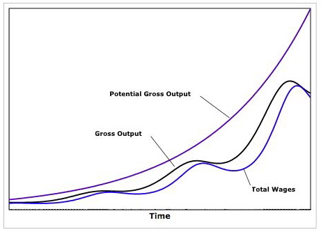
The figure below illustrates the movement of potential output (output at full employment), actual output and wages over time.

As can be seen the Goodwin model can generate endogenous fluctuations in economic activity without relying on extraneous assumptions of outside shocks, whether on the demand or supply side.

The model has been applied and extended by many economists since its first presentation in 1967.

Statistics

• 
  Wage share (blue line) and civilian employment population ratio (red line) in the United States
  According to the Goodwin model, the wage share is to be expected to lag behind the employment rate. This seems to be the case if only by a small time lag

See also

• Business cycle
• Richard M. Goodwin
• Harrod–Domar model
• Marxian economics
• Phillips curve

References

• Goodwin, Richard M. (1967), "A Growth Cycle", in C.H. Feinstein, editor, Socialism, Capitalism and Economic Growth. Cambridge: Cambridge University Press.
• Goodwin, Richard M., Chaotic Economic Dynamics, Oxford University Press, 1990.
• Flaschel, Peter, The Macrodynamics of Capitalism - Elements for a Synthesis of Marx, Keynes and Schumpeter. Second edition, Springer Verlag Berlin 2010. Chapter 4.3.