
Convective planetary boundary layer
The convective planetary boundary layer (CPBL), also known as the daytime planetary boundary layer (or simply convective boundary layer, CBL, when in context), is the part of the lower troposphere most directly affected by solar heating of the Earth's surface.[1]
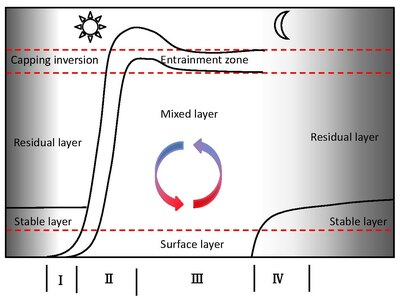
This layer extends from the Earth's surface to a capping inversion that typically locates at a height of 1–2 km by midafternoon over land. Below the capping inversion (10–60% of CBL depth, also called entrainment zone in the daytime), CBL is divided into two sub-layers: mixed layer (35–80% of CBL depth) and surface layer (5–10% of CBL depth). The mixed layer, the major part of CBL, has a nearly constant distribution of quantities such as potential temperature, wind speed, moisture and pollutant concentration because of strong buoyancy generated convective turbulent mixing.
Parameterization of turbulent transport is used to simulate the vertical profiles and temporal variation of quantities of interest, because of the randomness and the unknown physics of turbulence. However, turbulence in the mixed layer is not completely random, but is often organized into identifiable structures such as thermals and plumes in the CBL.[2] Simulation of these large eddies is quite different from simulation of smaller eddies generated by local shears in the surface layer. Non-local property of the large eddies should be accounted for in the parameterization.
Mean Characteristics[edit]
The mean characteristics of the three layers of the CBL are as follows.

(1) The Surface layer is a very shallow region close to the ground (bottom 5–10% of CBL). It is characterized by a superadiabatic lapse rate, moisture decrease with height and strong wind shear.[2] Almost all wind shear and all the potential temperature gradient in the CBL are confined in the surface layer.
(2) The Mixed layer composing the middle 35–80% of CBL[2] is characterized by conserved variables such as potential temperature, wind speed and moisture.
(3) The Entrainment zone (or Capping inversion) can be quite thick, averaging about 40% of the depth of the CBL. It is the region of statically stable air at the top of the mixed layer, where there is entrainment of free atmosphere air downward and overshooting thermals upward.[2] Potential temperature and wind speed have a sharp increase across the capping inversion, while moisture has a sharp decrease.
Evolution[edit]
CBL depth has a strong diurnal cycle with a four-phase process growth:[3]
(1) Formation of a shallow mixed layer: During the early morning the mixed layer is shallow and its depth increases slowly because of the strong nocturnal stable inversion capping.[4]
(2) Rapid growth: By the late morning, the cool nocturnal air has been warmed to a temperature near that of the residual layer, so the thermals penetrate rapidly upward during the second phase, allowing the top of the mixed layer to rise at rates of up to 1 km per 15 minutes.[4]
(3) Deep mixed layer of nearly constant thickness: When the thermals reach the capping inversion at the top of the residual layer, they meet resistance to vertical motion and the mixed layer growth rate rapidly decreases. During this third phase, which spans over most of the afternoon, the mixed layer depth is relatively constant. The lapse rate of temperature in the CBL is 1°/100 m.[4]
(4) Decay: Turbulence generated by buoyancy which drives the mixing decays after sunset and CBL collapses as well.
Turbulence in the CBL[edit]
In the atmospheric boundary layer, wind shear is responsible for the horizontal transport of heat, momentum, moisture and pollutants, while buoyancy dominates for the vertical mixing. Turbulences are generated by buoyancy and wind shear. If the buoyancy dominates over shear production, the boundary layer flow is in free convection. When shear generated turbulence is stronger than those generated by buoyancy, the flow is in forced convection.

In the surface layer, shear production always exceeds buoyancy production because of strong shear generated by surface drag. In the mixed layer, buoyancy generated by heating from the ground surface is the major driver of convective turbulence.[5] Radiative cooling from the cloud tops is also an effective driver of convection. The buoyancy generated turbulence peaks in the afternoon, hence the boundary layer flow is in free convection during most of the afternoon.
The up and downdrafts of boundary layer convection is the primary way in which the atmosphere moves heat, momentum, moisture, and pollutants between the Earth's surface and the atmosphere. Thus, boundary layer convection is important in the global climate modeling, numerical weather prediction, air-quality modeling and the dynamics of numerous mesoscale phenomena.
Mathematical simulation[edit]
Conservation equation[edit]
To quantitatively describe the variation of quantities in the CBL, we need to solve the conservation equations. The simplified form of the conservation equation for a passive scalar in typical CBL is

where is the mean of quantity , which could be water vapor mixing ratio , potential temperature , eastward-moving and northward-moving wind speed. is the vertical turbulent flux of .


We made several approximations to get the above simplified equation: ignore the body source, Bousinesq approximation, horizontal homogeneity and no subsidence. Bousinesq approximation is to ignore the density change due to pressure perturbation and keep the density change due to temperature change. This is a fairly good approximation in the CBL. The latter two approximations are not always effective in the real CBL. But this is acceptable in theoretical research. Observations show that turbulent mixing accounts for 50% of the total variation of potential temperature in a typical CBL.
However, due to the randomness of turbulences and our lack of knowledge about the exact physical behavior of it, parameterization of turbulent transport is needed in model simulation. Unlike shear dominated turbulence in the surface layer, large eddies associated with rise of warm air parcels that transport heat from hot to cold, regardless of the local gradient of the background environment exit in the mixed layer. Hence the non-local counter-gradient transport should be properly represented in the model simulation.
Several approaches are generally followed in numerical models to obtain the vertical profiles and temporal variations of quantities in CBL. Full mixing scheme for the whole CBL, local scheme for the shear dominated regions, non-local scheme and top-down and bottom up diffusion scheme for the buoyancy dominated mixed layer. In the full mixing scheme, all quantities are assumed to be uniformly distributed and the turbulent fluxes are assumed to be linearly related to height, with a jump at the top. In the local scheme, the turbulent flux is scaled by the local gradient of the quantity. In non-local scheme, the turbulence fluxes are related to known quantities at any number of grid points elsewhere in the vertical.[6] In top-down and bottom-up diffusion, the vertical profile is determined by diffusion from the two directions and the turbulent fluxes in sub-grid scale are derived from known quantities or their vertical derivatives at the same grid point.
Full mixing scheme[edit]
Full mixing is the simplest representation of CBL in some global models. Fluxes within this layer are assumed to decrease linearly with height, and the mean variables keep their vertical profile at each simulation time step.[7] All mean variables are uniformly distributed throughout the whole CBL and have a jump at the top of CBL. This simple model has been used in meteorology for a long time, and continues to be a popular approach in some global course resolution models.
Local closure[edit]
The local closure K-theory is a simple and effective scheme for shear dominated turbulent transport in the surface layer. K-theory assumes that mixing for heat, water vapor and pollutant concentration occurs only between adjacent layers of the CBL, and that the magnitude of mixing is determined by the eddy diffusion coefficient and local gradients of corresponding scalars .[8]


Where is an "eddy diffusion coefficient" for , which is typically taken as a function of a length scale and local vertical gradients of . For neutral condition, is parameterized using Mixing-Length Theory.


If a turbulent eddy moves a parcel of air upward by amount during which there is no mixing nor other changes in the value of within the parcel, then we define by


where is the von Karman constant empirically derived (0.35 or 0.4).

Mixing-length theory has its own limitation. The theory only applies to statically neutral condition.[9] It biases for statically stable and unstable conditions.
Mixing-length theory fails when the wind speed is uniformly distributed, people use knowledge of turbulent kinetic energy (TKE) to improve parameterization of eddy diffusion coefficient to account for large eddy transport in typical CBL. TKE gives us a measure of the intensity and effectiveness of turbulence and it could be measured accurately.

where is the dimensionless stability function, and is the TKE. The diagnostic equations used to obtain parameters and differ in different TKE closures.


Non-local closure[edit]
In buoyancy dominated regions, K-theory fails since it always yield unrealistic zero flux in a uniform environment. The non-local characteristics of large buoyancy eddies are accounted for by adding a non-local correction to the local scheme. The flux of any scalar can be described with[10]

where is a correction to the local gradient to represent the counter gradient flux transport of[clarification needed] large-scale eddies. This term is small in stable conditions, and is therefore neglected in such conditions. In unstable conditions, however, most transport is done by turbulent eddies with sizes on the order of the depth of the boundary layer.[10] In such cases,


where is the corresponding surface flux for a scalar , and is a coefficient of proportionality. is the mixed layer velocity scale defined from surface friction velocity and wind profile function at the surface layer top.


The eddy diffusivity for momentum is defined as

where is the von Karman constant, is the height above the ground, is the height of the boundary layer.

Compared to full mixing scheme, the non-local scheme significantly improves simulations of the vertical distributions for NO2 and O3, as evaluated in a study done in summer using aircraft measurements. It also reduces model biases at surface over the U.S. by 2-5 ppb for peak O3 (O3 concentration is 40-60ppb) in the afternoon, as evaluated using ground observations.[7]
Top-down and Bottom-up diffusion[edit]
The entrainment fluxes of quantities are not treated in the non-local scheme. In the top-down and bottom-up scheme, both the surface fluxes and the entrainment fluxes are represented. The mean scalar fluxes are the sum of the two fluxes[11]

Where is the height of mixed layer. and are the scalar flux at the top and bottom of CBL and scale as


Where and are


is the convective velocity scale . is the dimensionless gradient for the bottom up direction, a function of . is the dimensionless gradient for top-down. The vertical profile of and are provided in the Wyngaard et al., 1983 [11]


See also[edit]
References[edit]
- ^ Kaimal, J.C.; J.C. Wyngaard; D.A. Haugen; O.R. Cote; Y. Izumi (1976). "Turbulence Structure in the Convective Boundary Layer". Journal of the Atmospheric Sciences. 33 (11): 2152–2169. Bibcode:1976JAtS...33.2152K. doi:10.1175/1520-0469(1976)033<2152:tsitcb>2.0.co;2.
- ^ a b c d Stull, Rolald B. (1988). An Introduction to Boundary Layer Meteorology. Kluwer Academic Publishers. p. 441.
- ^ Stull, Rolald B. (1988). An Introduction to Boundary Layer Meteorology. Kluwer Academic Publishers. p. 451.
- ^ a b c Stull, Rolald B. (1988). An Introduction to Boundary Layer Meteorology. Kluwer Academic Publishers. p. 452.
- ^ Stull, Rolald B. (1988). An Introduction to Boundary Layer Meteorology. Kluwer Academic Publishers. p. 12.
- ^ Stull, Rolald B. (1988). An Introduction to Boundary Layer Meteorology. Kluwer Academic Publishers. p. 200.
- ^ a b Lin, Jin-Tai; Michael B. MaElroy (2010). "Impacts of boundary layer mixing on pollutant vertical profiles in the lower troposphere: Implications to satellite remote sensing". Atmospheric Environment. 44 (14): 1726–1739. Bibcode:2010AtmEn..44.1726L. doi:10.1016/j.atmosenv.2010.02.009.
- ^ Holtslag, A.A.M.; B.A. Boville (1993). "Local Versus Nonlocal Boundary-Layer Diffusion in a Global Climate Model". Journal of Climate. 6 (10): 1825–1842. Bibcode:1993JCli....6.1825H. doi:10.1175/1520-0442(1993)006<1825:lvnbld>2.0.co;2.
- ^ Stull, Rolald B. (1988). An Introduction to Boundary Layer Meteorology. Kluwer Academic Publishers. p. 208.
- ^ a b Hong, Song-You; Hua-Lu Pan (1996). "Nonlocal Boundary Layer Vertical Diffusion in a Medium-Range Forecast Model". Monthly Weather Review. 124 (10): 2322–2339. Bibcode:1996MWRv..124.2322H. doi:10.1175/1520-0493(1996)124<2322:nblvdi>2.0.co;2.
- ^ a b Wyngaard, John C.; Richard A. Brost (1983). "Top-down and bottom-up Diffusion of a scalar in the convective boundary layer". Journal of the Atmospheric Sciences. 1. 41 (1): 102–112. Bibcode:1984JAtS...41..102W. doi:10.1175/1520-0469(1984)041<0102:tdabud>2.0.co;2.