Overdetermined system

In mathematics, a system of equations is considered overdetermined if there are more equations than unknowns.^[1] An overdetermined system is almost always inconsistent (it has no solution) when constructed with random coefficients. However, an overdetermined system will have solutions in some cases, for example if some equation occurs several times in the system, or if some equations are linear combinations of the others.

The terminology can be described in terms of the concept of constraint counting. Each unknown can be seen as an available degree of freedom. Each equation introduced into the system can be viewed as a constraint that restricts one degree of freedom. Therefore the critical case occurs when the number of equations and the number of free variables are equal. For every variable giving a degree of freedom, there exists a corresponding constraint. The overdetermined case occurs when the system has been overconstrained — that is, when the equations outnumber the unknowns. In contrast, the underdetermined case occurs when the system has been underconstrained — that is, when the number of equations is fewer than the number of unknowns.

Systems of equations

An example in two dimensions

Consider the system of 3 equations and 2 unknowns (x₁ and x₂), which is overdetermined because 3>2, and which corresponds to Diagram #1:

$2x_{1}+x_{2}=-1$

$-3x_{1}+x_{2}=-2$

$-x_{1}+x_{2}=1$ .

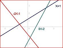
There is one solution for each pair of linear equations: for the first and second equations (0.2, −1.4), for the first and third (−2/3, 1/3), and for the second and third (1.5, 2.5). However there is no solution that satisfies all three simultaneously. Diagrams #2 and 3 show other configurations that are inconsistent because no point is on all of the lines. Systems of this variety are deemed inconsistent.

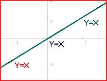
The only cases where the overdetermined system does in fact have a solution are demonstrated in Diagrams #4, 5, and 6. These exceptions can occur only when the overdetermined system contains enough linearly dependent equations that the number of independent equations does not exceed the number of unknowns. Linear dependence means that some equations can be obtained from linearly combining other equations. For example, y = x + 1 and 2y = 2x + 2 are linearly dependent equations because the second one can be obtained by taking twice the first one.

Matrix form

Any system of linear equations can be written as a matrix equation. The previous system of equations can be written as follows:

{\begin{bmatrix}2&1\\-3&1\\-1&1\\\end{bmatrix}}{\begin{bmatrix}X_{1}\\X_{2}\\\end{bmatrix}}={\begin{bmatrix}-1\\-2\\1\\\end{bmatrix}}

Notice that the rows of the matrix (corresponding to equations) outnumber the columns (corresponding to unknowns), meaning that the system is overdetermined. In linear algebra the concepts of row space, column space and null space are important for determining the properties of matrices. The informal discussion of constraints and degrees of freedom above relates directly to these more formal concepts.

Homogeneous case

The homogeneous case (in which all constant terms are zero) is always consistent (because there is a trivial, all-zero solution). There are two cases, depending on the number of linearly dependent equations: either there is just the trivial solution, or there is the trivial solution plus an infinite set of other solutions.

Consider the system of linear equations: L_i = 0 for 1 ≤ i ≤ M, and variables X₁, X₂, ..., X_N, where each L_i is a weighted sum of the X_is. Then X₁ = X₂ = ... = X_N = 0 is always a solution. When M < N the system is underdetermined and there are always an infinitude of further solutions. In fact the dimension of the space of solutions is always at least N − M.

For M ≥ N, there may be no solution other than all values being 0. There will be an infinitude of other solutions only when the system of equations has enough dependencies (linearly dependent equations) that the number of independent equations is at most N − 1. But with M ≥ N the number of independent equations could be as high as N, in which case the trivial solution is the only one.

Non-homogeneous case

In systems of linear equations, L_i=c_i for 1 ≤ i ≤ M, in variables X₁, X₂, ..., X_N the equations are sometimes linearly dependent; in fact the number of linearly independent equations cannot exceed N+1. We have the following possible cases for an overdetermined system with N unknowns and M equations (M>N).

M = N+1 and all M equations are linearly independent. This case yields no solution. Example: x = 1, x = 2.
M > N but only K equations (K < M and K ≤ N+1) are linearly independent. There exist three possible sub-cases of this:
- K = N+1. This case yields no solutions. Example: 2x = 2, x = 1, x = 2.
- K = N. This case yields either a single solution or no solution, the latter occurring when the coefficient vector of one equation can be replicated by a weighted sum of the coefficient vectors of the other equations but that weighted sum applied to the constant terms of the other equations does not replicate the one equation's constant term. Example with one solution: 2x = 2, x = 1. Example with no solution: 2x + 2y = 2, x + y = 1, x + y = 3.
- K < N. This case yields either infinitely many solutions or no solution, the latter occurring as in the previous sub-case. Example with infinitely many solutions: 3x + 3y = 3, 2x + 2y = 2, x + y = 1. Example with no solution: 3x + 3y + 3z = 3, 2x + 2y + 2z = 2, x + y + z = 1, x + y + z = 4.

These results may be easier to understand by putting the augmented matrix of the coefficients of the system in row echelon form by using Gaussian elimination. This row echelon form is the augmented matrix of a system of equations that is equivalent to the given system (it has exactly the same solutions). The number of independent equations in the original system is the number of non-zero rows in the echelon form. The system is inconsistent (no solution) if and only if the last non-zero row in echelon form has only one non-zero entry that is in the last column (giving an equation 0 = c where c is a non-zero constant). Otherwise, there is exactly one solution when the number of non-zero rows in echelon form is equal to the number of unknowns, and there are infinitely many solutions when the number of non-zero rows is lower than the number of variables.

Putting it another way, according to the Rouché–Capelli theorem, any system of equations (overdetermined or otherwise) is inconsistent if the rank of the augmented matrix is greater than the rank of the coefficient matrix. If, on the other hand, the ranks of these two matrices are equal, the system must have at least one solution. The solution is unique if and only if the rank equals the number of variables. Otherwise the general solution has k free parameters where k is the difference between the number of variables and the rank; hence in such a case there are an infinitude of solutions.

Exact solutions

All exact solutions can be obtained, or it can be shown that none exist, using matrix algebra. See System of linear equations#Matrix solution.

Approximate solutions

The method of ordinary least squares can be used to find an approximate solution to overdetermined systems. For the system $Ax=b,$ the least squares formula is obtained from the problem

\min _{x}\Vert Ax-b\Vert ,

the solution of which can be written with the normal equations,^[2]

x=(A^{\mathrm {T} }A)^{-1}A^{\mathrm {T} }b,

where ${\mathrm {T} }$ indicates a matrix transpose, provided $(A^{\mathrm {T} }A)^{-1}$ exists (that is, provided A has full column rank). With this formula an approximate solution is found when no exact solution exists, and it gives an exact solution when one does exist. However, to achieve good numerical accuracy, using the QR factorization of A to solve the least squares problem is preferred.^[3]

In general use

The concept can also be applied to more general systems of equations, such as systems of polynomial equations or partial differential equations. In the case of the systems of polynomial equations, it may happen that an overdetermined system has a solution, but that no one equation is a consequence of the others and that, when removing any equation, the new system has more solutions. For example, $(x-1)(x-2)=0,(x-1)(x-3)=0$ has the single solution $x=1,$ but each equation by itself has two solutions.

References

^ "Planet Math, Overdetermined".
^ Anton, Howard; Rorres,, Chris (2005). Elementary Linear Algebra (9th ed.). John Wiley and Sons, Inc. ISBN 978-0-471-66959-3.{{cite book}}: CS1 maint: extra punctuation (link)
^ Trefethen, Lloyd; Bau, III, David (1997). Numerical Linear Algebra. ISBN 978-0898713619.

[1] "Planet Math, Overdetermined".

[2] Anton, Howard; Rorres,, Chris (2005). Elementary Linear Algebra (9th ed.). John Wiley and Sons, Inc. ISBN 978-0-471-66959-3.{{cite book}}: CS1 maint: extra punctuation (link)

[3] Trefethen, Lloyd; Bau, III, David (1997). Numerical Linear Algebra. ISBN 978-0898713619.

[1]

[2]

[3]