Zero-suppressed decision diagram

A zero-suppressed decision diagram (ZSDD or ZDD) is a particular kind of binary decision diagram (BDD) with fixed variable ordering. This data structure provides a canonically compact representation of sets, particularly suitable for certain combinatorial problems. Recall the Ordered Binary Decision Diagram (OBDD) reduction strategy, i.e. a node is replaced with one of its children if both out-edges point to the same node. In contrast, a node in a ZDD is replaced with its negative child if its positive edge points to the terminal node 0. This provides an alternative strong normal form, with improved compression of sparse sets. It is based on a reduction rule devised by Shin-ichi Minato in 1993.

Background[edit]

In a binary decision diagram, a Boolean function can be represented as a rooted, directed, acyclic graph, which consists of several decision nodes and terminal nodes. In 1993, Shin-ichi Minato from Japan modified Randal Bryant's BDDs for solving combinatorial problems. His "Zero-Suppressed" BDDs aim to represent and manipulate sparse sets of bit vectors. If the data for a problem are represented as bit vectors of length n, then any subset of the vectors can be represented by the Boolean function over n variables yielding 1 when the vector corresponding to the variable assignment is in the set.

According to Bryant, it is possible to use forms of logic functions to express problems involving sum-of-products. Such forms are often represented as sets of "cubes", each denoted by a string containing symbols 0, 1, and -. For instance, the function $({\bar {x}}_{1}\land x_{2})\lor ({\bar {x}}_{2}\oplus x_{3})$ can be illustrated by the set $\{01-,-11,-00\}$ . By using bits 10, 01, and 00 to denote symbols 1, 0, and – respectively, one can represent the above set with bit vectors in the form of $\{011000,001010,000101\}$ . Notice that the set of bit vectors is sparse, in that the number of vectors is fewer than 2ⁿ, which is the maximum number of bit vectors, and the set contains many elements equal to zero. In this case, a node can be omitted if setting the node variable to 1 causes the function to yield 0. This is seen in the condition that a 1 at some bit position implies that the vector is not in the set. For sparse sets, this condition is common, and hence many node eliminations are possible.

Minato has proved that ZDDs are especially suitable for combinatorial problems, such as the classical problems in two-level logic minimization, knight's tour problem, fault simulation, timing analysis, the N-queens problem, as well as weak division. By using ZDDs, one can reduce the size of the representation of a set of n-bit vectors in OBDDs by at most a factor of n. In practice, the optimization is statistically significant.

Definitions[edit]

We define a Zero-Suppressed Decision Diagram (ZDD) to be any directed acyclic graph such that:

1. A terminal node is either:

The special ⊤ node which represents the unit family $\{\emptyset \}$ (i.e., the empty set), or
The special ⊥ node which represents the empty family $\emptyset$ .

2. Each nonterminal node satisfies the following conditions:

a. The node is labelled with a positive integer v. This label does not have to be unique.

b. The node has an out-degree of 2. One of the outgoing edges is named "LO", and the other "HI". (In diagrams, one may draw dotted lines for LO edges and solid lines for HI edges)

c. A destination node is either terminal or labelled with an integer strictly larger than v. Thus one can omit arrowheads in diagrams because the edge directions can be inferred from the labels.

d. The HI edge never points to the ⊥ node.

3. There is exactly one node with zero in-degree—the root node. The root node is either terminal or labelled by the smallest integer in the diagram.

4. If two nodes have the same label, then their LO or HI edges point to different nodes. In other words, there are no redundant nodes.

We call Z an unreduced ZDD, if a HI edge points to a ⊥ node or condition 4 fails to hold. In computer programs, Boolean functions can be expressed in bits, so the ⊤ node and ⊥ node can be represented by 1 and 0. From the definition above, we can represent combination sets efficiently by applying two rules to the BDDs:

1.Eliminate all the nodes whose 1-edge points to the 0-terminal node (Figure 1). Then connect the edge to the other subgraph directly.

2.Share all equivalent sub-graphs the same as for original BDDs.

If the number and the order of input variables are fixed, a zero-suppressed BDD represents a Boolean function uniquely (as proved in Figure 2, it is possible to use a BDD to represent a Boolean binary tree).

Representing a family of sets[edit]

Let F be a ZDD. Let v be its root node. Then:

1. If v = ⊥ , then there can be no other nodes, and F represents Ø, the empty family.

2. If v = ⊤, then there can be no other nodes, and F represents the family containing just the empty set { Ø }. We call this a unit family, and denote it by .

3. If v has two children. Let v0 be the LO node, and v1 be the HI node. Let Fi be the family represented by the ZDD rooted at vi, which can be shown by proof of induction. Then F represents the family

F_{0}\cup \{\alpha \cup \{v\}\mid \alpha \in F_{1}\}

One may represent the LO branch as the sets in F that don't contain v: $F_{0}=\{\alpha :\alpha \in F,v\notin \alpha \}$

And the HI branch as the sets in F that do contain v: $F_{1}=\{\alpha \smallsetminus \{v\}:\alpha \in F,v\in \alpha \}$

Example[edit]

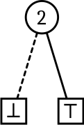Figure 3
Figure 4
Figure 5
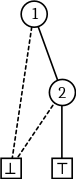Figure 6

Figure 3: The family $\emptyset \cup \{\emptyset \cup \{2\}\}=\{\{2\}\}$ . We may call this $e_{2}$ , an elementary family. Elementary families consist of the form $\{\{n\}\}$ , and are denoted by $e_{n}$ .

Figure 4: The family $\{\emptyset \}\cup \{\emptyset \cup \{2\}\}=\{\emptyset ,\{2\}\}$

Figure 5: The family $\{\{2\}\}\cup \{\emptyset \cup \{1\}\}=\{\{1\},\{2\}\}$

Figure 6: The family $\{\{1\}\cup \{2\}\}=\{\{1,2\}\}$

Features[edit]

One feature of ZDDs is that the form does not depend on the number of input variables as long as the combination sets are the same. It is unnecessary to fix the number of input variables before generating graphs. ZDDs automatically suppress the variables for objects which never appear in combination, hence the efficiency for manipulating sparse combinations. Another advantage of ZDDs is that the number of 1-paths in the graph is exactly equal to the number of elements in the combination set. In original BDDs, the node elimination breaks this property. Therefore, ZDDs are better than simple BDDs to represent combination sets. It is, however, better to use the original BDDs when representing ordinary Boolean functions, as shown in Figure 7.

Basic operations[edit]

Here we have the basic operations for ZDDs, as they are slightly different from those of the original BDDs. One may refer to Figure 8 for examples generated from the table below.

Empty() returns ø (empty set)

Base() returns{0}

Subset1(P, var) returns the subset of P such as var = 1

Subset0(P, var) returns the subset of P such as var = 0

Change(P, var) returns P when var is inverted

Union(P, Q) returns (

P\cup Q

)

Intsec(P, Q) returns (

P\cap Q

)

Diff(P, Q) returns (

P-Q

)

Count(P) returns

\left\vert P\right\vert

. (number of elements)

In ZDDs, there is no NOT operation, which is an essential operation in original BDDs. The reason is that the complement set ${\bar {P}}$ cannot be computed without defining the universal set $U$ . In ZDDs, ${\bar {P}}$ can be computed as Diff(U, P).

Algorithms[edit]

Suppose $\left\vert P\right\vert =\left\vert P_{0}\right\vert +\left\vert P_{1}\right\vert$ , we can recursively compute the number of sets in a ZDD, enabling us to get the 34th set out a 54-member family. Random access is fast, and any operation possible for an array of sets can be done with efficiency on a ZDD.

According to Minato, the above operations for ZDDs can be executed recursively like original BDDs. To describe the algorithms simply, we define the procedure Getnode(top, P0, P1) that returns a node for a variable top and two subgraphs P0 and P1. We may use a hash table, called uniq-table, to keep each node unique. Node elimination and sharing are managed only by Getnode().

 Getnode (top, P0, P1) {
   if (P1 == ø) return P0; /* node elimination */
   P = search a node with (top, P0, P1 ) in uniq-table; if (P exist) return P; /* node sharing */
   P = generate a node with (top, P0, P1 );
   append P to the uniq-table;
   return P; 
 }

Using Getnode(), we can then represent other basic operations as follows:

 Subset1 (P, var) {
   if (P.top < var) return ø; 
   if (P.top == var) return P1; 
   if (P.top > var)
     return Getnode (P.top, Subset1(P0, var), Subset1(P1, var));
 }

 Subset0 (P, var) {
   if (P.top < var) return ø; 
   if (P.top == var) return P0; 
   if (P.top > var)
     return Getnode (P.top, Subset0(P0, var), Subset0(P1, var));
 }

 Change (P, var) {
   if (P.top < var) return Getnode (var, ø, P); 
   if (P.top == var) return Getnode (var, P1, P0);
   if (P.top > var)
     return Getnode (P.top, Change(P0, var), Change(P1, var));
 }

 Union (P, Q) {
   if (P == ø) return Q; 
   if (Q == ø) return P;
   if (P == Q) return P;
   if (P.top > Q.top) return Getnode (P.top, Union(P0, Q), P1);
   if (P.top < Q.top) return Getnode (Q.top, Union(P, Q0), Q1);
   if (P.top == Q.top) 
     return Getnode (P.top, Union(P0, Q0), Union(P1, Q1));
 }

 Intsec (P, Q) {
   if (P == ø) return ø; 
   if (Q == ø) return ø;
   if (P == Q) return P;
   if (P.top > Q.top) return Intsec(P0, Q);
   if (P.top < Q.top) return Intsec (P, Q0);
   if (P.top == Q.top) 
     return Getnode (P.top, Intsec(P0, Q0), Intsec(P1, Q1));
 }

 Diff (P, Q) {
   if (P == ø) return ø; 
   if (Q == ø) return P;
   if (P == Q) return ø;
   if (P.top > Q.top) return Getnode(P.top, Diff(P0, Q), P1;)
   if (P.top < Q.top) return Diff(P, Q0);
   if (P.top == Q.top) 
     return Getnode (P.top, Diff(P0, Q0), Diff(P1, Q1));
 }

 Count (P) {
   if (P == ø) return 0; 
   if (P == {ø}) return 1;
     return Count(P0) + Count(P1);
 }

These algorithms take an exponential time for the number of variables in the worst case; however, we can improve the performance by using a cache that memorizes results of recent operations in a similar fashion in BDDs. The cache prevents duplicate executions for equivalent sub-graphs. Without any duplicates, the algorithms can operate in a time that is proportional to the size of graphs, as shown in Figure 9 and 10.

Application[edit]

ZDDs as dictionaries[edit]

ZDDs can be used to represent the five-letter words of English, the set WORDS (of size 5757) from the Stanford GraphBase for instance. One way to do this is to consider the function $f(x_{1},...,x_{25})$ that is defined to be 1 if and only if the five numbers $(x_{1},...,x_{5})_{2}$ , $(x_{6},...,x_{10})_{2}$ , ..., $(x_{21},...,x_{25})_{2}$ encode the letters of an English word, where $a=(00001)_{2}$ , ..., $z=(11010)_{2}$ . For example, $f(0,0,1,1,1,0,1,1,1,1,0,1,1,1,1,0,0,1,1,0,1,1,0,0,x_{25})=x_{25}$ . The function of 25 variables has Z(f) = 6233 nodes – which is not too bad for representing 5757 words. Compared to binary trees, tries, or hash tables, a ZDD may not be the best to complete simple searches, yet it is efficient in retrieving data that is only partially specified, or data that is only supposed to match a key approximately. Complex queries can be handled with ease. Moreover, ZDDs do not involve as many variables. In fact, by using a ZDD, one can represent those five letter words as a sparse function $F(a_{1},...,z_{1},a_{2},...,z_{2},...,a_{5},...,z_{5})$ that has 26×5 = 130 variables, where variable $a_{2}$ for example determines whether the second letter is "a". To represent the word "crazy", one can make F true when $c_{1}=r_{2}=a_{3}=z_{4}=y_{5}=1$ and all other variables are 0. Thus, F can be considered as a family consisting of the 5757 subsets $\{w_{1},h_{2},i_{3},c_{4},h_{5}\}$ , etc. With these 130 variables the ZDD size Z(F) is in fact 5020 instead of 6233. According to Knuth, the equivalent size of B(F) using a BDD is 46,189—significantly larger than Z(F). In spite of having similar theories and algorithms, ZDDs outperform BDDs for this problem with quite a large margin. Consequently, ZDDs allow us to perform certain queries that are too onerous for BDDs. Complex families of subset can readily be constructed from elementary families. To search words containing a certain pattern, one may use family algebra on ZDDs to compute $(F/P)\sqcup P$ where P is the pattern, e.g $a_{1}\sqcup h_{3}\sqcup e_{5}$ .

ZDDs to represent simple paths[edit]

One may use ZDDs to represent simple paths in an undirected graph. For example, there are 12 ways to go from the upper left corner of a three by three grid (shown in Figure 11) to the lower right corner, without visiting any point twice.

Figure 12: 12 possible paths to go one corner to the other diagonal corner

These paths can be represented by the ZDD shown in Figure 13, in which each node mn represents the question "does the path include the arc between m and n?" So, for example, the LO branch between 13 and 12 indicates that if the path does not include the arc from 1 to 3, the next thing to ask is if it includes the arc from 1 to 2. The absence of a LO branch leaving node 12 indicates that any path that does not go from 1 to 3 must therefore go from 1 to 2. (The next question to ask would be about the arc between 2 and 4.) In this ZDD, we get the first path in Figure 12 by taking the HI branches at nodes 13, 36, 68, and 89 of the ZDD (LO branches that simply go to ⊥ are omitted). Although the ZDD in Figure 13 may not seem significant by any means, the advantages of a ZDD become obvious as the grid gets larger. For example, for an eight by eight grid, the number of simple paths from corner to corner turns out to be 789,360,053,252 (Knuth). The paths can be illustrated with 33580 nodes using a ZDD.

A real world example for simple paths was proposed by Randal Bryant, "Suppose I wanted to take a driving tour of the Continental U.S., visiting all of the state capitols, and passing through each state only once. What route should I take to minimize the total distance?" Figure 14 shows an undirected graph for this roadmap, the numbers indicating the shortest distances between neighboring capital cities. The problem is to choose a subset of these edges that form a Hamiltonian path of smallest total length. Every Hamiltonian path in this graph must either start or end at Augusta, Maine(ME). Suppose one starts in CA. One can find a ZDD that characterizes all paths from CA to ME. According to Knuth, this ZDD turns out to have only 7850 nodes, and it effectively shows that exactly 437,525,772,584 simple paths from CA to ME are possible. By number of edges, the generating function is

                       $4z^{11}+124z^{12}+1539z^{13}+...+33385461z^{46}+2707075z^{47}$ ;

so the longest such paths are Hamiltonian, with a size of 2,707,075. ZDDs in this case, are efficient for simple paths and Hamiltonian paths.

The eight-queens problem[edit]

Define 64 input variables to represent the squares on a chess board. Each variable denotes the presence or absence of a queen on that square. Consider that,

In a particular column, only one variable is "1".
In a particular row, only one variable is "1".
On a particular diagonal line, one or no variable is "1".

Although one can solve this problem by constructing OBDDs, it is more efficient to use ZDDs. Constructing a ZDD for the 8-Queens problem requires 8 steps from S1 to S8. Each step can be defined as follows:

S1: Represents all choices of putting a queen at the first row.

S2: Represents all choices of putting a queen at the second row so as not to violate the first queen.

S3: Represents all choices of putting a queen at the third row so that it does not violate the previous queens.

…

S8: Represents all choices of putting a queen at the eighth row so that it does not violate the previous queens.

The ZDD for S8 consists of all potential solutions of the 8-Queens problem. For this particular problem, caching can significantly improve the performance of the algorithm. Using cache to avoid duplicates can improve the N-Queens problems up to 4.5 times faster than using only the basic operations (as defined above), shown in Figure 10.

The knight's tour problem[edit]

The Knight's tour problem has a historical significance. The knight's graph contains n² vertices to depict the squares of the chessboard. The edges illustrate the legal moves of a knight. The knight can visit each square of the board exactly once. Olaf Schröer, M. Löbbing, and Ingo Wegener approached this problem, namely on a board, by assigning Boolean variables for each edge on the graph, with a total of 156 variables to designate all the edges. A solution of the problem can be expressed by a 156-bit combination vector. According to Minato, the construction of a ZDD for all solutions is too large to solve directly. It is easier to divide and conquer. By dividing the problems into two parts of the board, and constructing ZDDs in subspaces, one can solve The Knight's tour problem with each solution containing 64 edges. However, since the graph is not very sparse, the advantage of using ZDDs is not so obvious.

Fault simulation[edit]

N. Takahashi et al suggested a fault simulation method given multiple faults by using OBDDs. This deductive method transmits the fault sets from primary inputs to primary outputs, and captures the faults at primary outputs. Since this method involves unate cube set expressions, ZDDs are more efficient. The optimizations from ZDDs in unate cube set calculations indicate that ZDDs could be useful in developing VLSI CAD systems and in a myriad of other applications.

Available packages[edit]

CUDD: A BDD package written in C that implements BDDs and ZBDDs, University of Colorado, Boulder
JDD, A java library that implements common BDD and ZBDD operations
Graphillion, A ZDD software implementation based on Python
[1], A CWEB ZDD implementation by Donald Knuth.

References[edit]

External links[edit]

Lynn, Ben. "ZDDs." ZDDs - Introduction, Stanford University, 2005, crypto.stanford.edu/pbc/notes/zdd/
Donald Knuth, Fun With Zero-Suppressed Binary Decision Diagrams (ZDDs) (video lecture, 2008)
Minato Shin-ichi, Counting paths in graphs (fundamentals of ZDD) (video illustration produced on Miraikan)