
Reed–Solomon error correction: Difference between revisions
infobox updated |
|||
| Line 4: | Line 4: | ||
| image_caption = |
| image_caption = |
||
| namesake = [[Irving S. Reed]] and [[Gustave Solomon]] |
| namesake = [[Irving S. Reed]] and [[Gustave Solomon]] |
||
| |
| type = [[Linear block code]] |
||
| block_length = |
| block_length = <math>n</math> |
||
| message_length = |
| message_length = <math>k</math> |
||
| |
| rate = <math>k/n</math> |
||
| distance = <math>n-k+1</math> |
|||
| alphabet_size = ''q'' = ''p''<sup>''m''</sup> (''p'' prime) |
|||
| alphabet_size = <math>q</math> |
|||
| notation = [''n'', ''k'', ''n'' - ''k'' + 1]<sub>''q''</sub>-code |
|||
| notation = <math>[n,k,n-k+1]_q</math> |
|||
| decoding = [[Berlekamp–Massey algorithm|Berlekamp–Massey]]<br>[[Euclidean algorithm|Euclidean]]<br>''et al.'' |
|||
| properties = [[maximum distance separable code|Maximum-distance separable code]] |
|||
}} |
}} |
||
| Line 101: | Line 100: | ||
The above properties of Reed–Solomon codes make them especially well-suited to applications where errors occur in [[burst error|burst]]s. This is because it does not matter to the code how many bits in a symbol are in error — if multiple bits in a symbol are corrupted it only counts as a single error. Conversely, if a data stream is not characterized by error bursts or drop-outs but by random single bit errors, a Reed–Solomon code is usually a poor choice compared to a binary code. |
The above properties of Reed–Solomon codes make them especially well-suited to applications where errors occur in [[burst error|burst]]s. This is because it does not matter to the code how many bits in a symbol are in error — if multiple bits in a symbol are corrupted it only counts as a single error. Conversely, if a data stream is not characterized by error bursts or drop-outs but by random single bit errors, a Reed–Solomon code is usually a poor choice compared to a binary code. |
||
The Reed–Solomon code, like the [[convolutional code]], is a transparent code. This means that if the channel symbols have been [[bitwise NOT|inverted]] somewhere along the line, the decoders will still operate. The result will be the inversion of the original data. However, the Reed–Solomon code loses its transparency when the code is shortened. The "missing" bits in a shortened code need to be filled by either zeros or |
The Reed–Solomon code, like the [[convolutional code]], is a transparent code. This means that if the channel symbols have been [[bitwise NOT|inverted]] somewhere along the line, the decoders will still operate. The result will be the inversion of the original data. However, the Reed–Solomon code loses its transparency when the code is shortened. The "missing" bits in a shortened code need to be filled by either zeros or ones, depending on whether the data is complemented or not. (To put it another way, if the symbols are inverted, then the zero-fill needs to be inverted to a one-fill.) For this reason it is mandatory that the sense of the data (i.e., true or complemented) be resolved before Reed–Solomon decoding. |
||
== Error correction algorithms == |
|||
=== Theoretical decoder === |
|||
{{Harvtxt|Reed|Solomon|1960}} described a theoretical decoder that corrected errors by finding the most popular message polynomial. The decoder for a RS <math>(n,k)</math> code would look at all possible subsets of <math>k</math> symbols from the set of <math>n</math> symbols that were received. For the code to be correctable in general, at least <math>k</math> symbols had to be received correctly, and <math>k</math> symbols are needed to interpolate the message polynomial. The decoder would interpolate a message polynomial for each subset, and it would keep track of the resulting polynomial candidates. The most popular message is the corrected result. Unfortunately, there are a lot of subsets, so the algorithm is impractical. The number of subsets is the [[binomial coefficient]], <math>\textstyle \binom{n}{k} = {n! \over (n-k)! k!}</math>, and the number of subsets is infeasible for even modest codes. For a <math>(255,249)</math> code that can correct 3 errors, the naive theoretical decoder would examine 359 billion subsets. <!-- = 255 * 254 * 253 * 252 * 251 * 250 / 720 rounded down; could say 360B --> The RS code needed a practical decoder. |
|||
=== Peterson decoder === |
|||
{{main|BCH code#Peterson–Gorenstein–Zierler algorithm|l1=Peterson–Gorenstein–Zierler algorithm}} |
|||
{{Harvtxt|Peterson|1960}} developed a practical decoder based on syndrome decoding. {{Harv|Welch|1997|p=10}} Berlekamp (below) would improve on that decoder. |
|||
====Syndrome decoding==== |
|||
The transmitted message is viewed as the coefficients of a polynomial ''s''(''x'') that is divisible by a generator polynomial ''g''(''x''). {{Harvtxt|Welch|1997|p=5}} |
|||
:<math>s(x) = \sum_{i = 0}^{n-1} c_i x^i</math> |
|||
:<math>g(x) = \prod_{j=1}^{n-k} (x - \alpha^j), </math> |
|||
where ''α'' is a primitive root. |
|||
Since ''s''(''x'') is divisible by generator ''g''(''x''), it follows that |
|||
:<math>s(\alpha^i) = 0, \ i=1,2,\ldots,n-k</math> |
|||
The transmitted polynomial is corrupted in transit by an error polynomial ''e''(''x'') to produce the received polynomial ''r''(''x''). |
|||
:<math>r(x) = s(x) + e(x)</math> |
|||
:<math>e(x) = \sum_{i=0}^{n-1} e_i x^i </math> |
|||
where ''e<sub>i</sub>'' is the coefficient for the ''i''-th power of ''x''. Coefficient ''e<sub>i</sub>'' will be zero if there is no error at that power of ''x'' and nonzero if there is an error. If there are ''ν'' errors at distinct powers ''i<sub>k</sub>'' of ''x'', then |
|||
:<math>e(x) = \sum_{k=1}^\nu e_{i_k} x^{i_k}</math> |
|||
The goal of the decoder is to find ''ν'', the positions ''i<sub>k</sub>'', and the error values at those positions. |
|||
The syndromes ''S''<sub>''j''</sub> are defined as |
|||
:<math> |
|||
\begin{align} |
|||
S_j &= r(\alpha^j) = s(\alpha^j) + e(\alpha^j) = 0 + e(\alpha^j) = e(\alpha^j), \ j=1,2,\ldots,n-k \\ |
|||
&= \sum_{k=1}^{\nu} e_{i_k} \left( \alpha^{j} \right)^{i_k} |
|||
\end{align} |
|||
</math> |
|||
The advantage of looking at the syndromes is that the message polynomial drops outs. |
|||
====Error locators and error values==== |
|||
<!-- There's confusion between index k and the k in (n,k). Literature also has confusion? Or does it use kappa? --> |
|||
For convenience, define the '''error locators''' ''X<sub>k</sub>'' and '''error values''' ''Y<sub>k</sub>'' as: |
|||
:<math> X_k = \alpha^{i_k}, \ Y_k = e_{i_k} </math> |
|||
Then the syndromes can be written in terms of the error locators and error values as |
|||
:<math> S_j = \sum_{k=1}^{\nu} Y_k X_k^{j} </math> |
|||
The syndromes give a system of ''n'' − ''k'' ≥ 2''ν'' equations in 2''ν'' unknowns, but that system of equations is nonlinear in the ''X<sub>k</sub>'' and does not have an obvious solution. However, if the ''X<sub>k</sub>'' were known (see below), then the syndrome equations provide a linear system of equations that can easily be solved for the ''Y<sub>k</sub>'' error values. |
|||
<!-- |
|||
Vandermonde comment. Matrix equation --> |
|||
:<math>\begin{bmatrix} |
|||
X_1^1 & X_2^1 & \cdots & X_\nu^1 \\ |
|||
X_1^2 & X_2^2 & \cdots & X_\nu^2 \\ |
|||
\vdots & \vdots && \vdots \\ |
|||
X_1^{n-k} & X_2^{n-k} & \cdots & X_\nu^{n-k} \\ |
|||
\end{bmatrix} |
|||
\begin{bmatrix} |
|||
Y_1 \\ Y_2 \\ \vdots \\ Y_\nu |
|||
\end{bmatrix} |
|||
= |
|||
\begin{bmatrix} |
|||
S_1 \\ S_2 \\ \vdots \\ S_{n-k} |
|||
\end{bmatrix} |
|||
</math> |
|||
Consequently, the problem is finding the ''X<sub>k</sub>''. |
|||
====Error locator polynomial==== |
|||
Peterson found a linear recurrence relation that gave rise to a system of linear equations. {{Harv|Welch|1997|p=10}} |
|||
Solving those equations identifies the error locations. |
|||
<!-- |
|||
Derivation here. Massey has formal power series gymnastics. --> |
|||
Define the '''error locator polynomial''' Λ(''x'') as |
|||
:<math>\Lambda(x) = \prod_{k=1}^\nu (1 - x X_k ) = 1 + \Lambda_1 x^1 + \Lambda_2 x^2 + \cdots + \Lambda_\nu x^\nu</math> |
|||
The zeros of Λ(''x'') are the reciprocals <math>X_k^{-1}</math>: |
|||
:<math> \Lambda(X_k^{-1}) = 0 </math> |
|||
:<math>\Lambda(X_k^{-1}) = 1 + \Lambda_1 X_k^{-1} + \Lambda_2 X_k^{-2} + \cdots + \Lambda_\nu X_k^{-\nu} = 0 </math> |
|||
Multiply both sides by <math>Y_k X_k^{j+\nu}</math> and it will still be zero. |
|||
:<math> |
|||
\begin{align} |
|||
& Y_k X_k^{j+\nu} \Lambda(X_k^{-1}) = 0. \\ |
|||
\text{Hence } & Y_k X_k^{j+\nu} + \Lambda_1 Y_k X_k^{j+\nu} X_k^{-1} + \Lambda_2 Y_k X_k^{j+\nu} X_k^{-2} + \cdots + \Lambda_{\nu} Y_k X_k^{j+\nu} X_k^{-\nu} = 0, \\ |
|||
\text{and so } & Y_k X_k^{j+\nu} + \Lambda_1 Y_k X_k^{j+\nu-1} + \Lambda_2 Y_k X_k^{j+\nu -2} + \cdots + \Lambda_{\nu} Y_k X_k^j = 0 \\ |
|||
\end{align} |
|||
</math> |
|||
Sum for ''k'' = 1 to ''ν'' |
|||
:<math>\begin{align} |
|||
& \sum_{k=1}^\nu ( Y_k X_k^{j+\nu} + \Lambda_1 Y_k X_k^{j+\nu-1} + \Lambda_2 Y_k X_k^{j+\nu -2} + \cdots + \Lambda_{\nu} Y_k X_k^{j} ) = 0 \\ |
|||
& \sum_{k=1}^\nu ( Y_k X_k^{j+\nu} ) + \Lambda_1 \sum_{k=1}^\nu (Y_k X_k^{j+\nu-1}) + \Lambda_2 \sum_{k=1}^\nu (Y_k X_k^{j+\nu -2}) + \cdots + \Lambda_\nu \sum_{k=1}^\nu ( Y_k X_k^j ) = 0 |
|||
\end{align}</math> |
|||
This reduces to |
|||
:<math> S_{j + \nu} + \Lambda_1 S_{j+\nu-1} + \cdots + \Lambda_{\nu-1} S_{j+1} + \Lambda_{\nu} S_j = 0 \, </math> |
|||
:<math> S_j \Lambda_{\nu} + S_{j+1}\Lambda_{\nu-1} + \cdots + S_{j+\nu-1} \Lambda_1 = - S_{j + \nu} \ </math> |
|||
This yields a system of linear equations that can be solved for the coefficients Λ<sub>''i''</sub> of the error location polynomial: |
|||
:<math>\begin{bmatrix} |
|||
S_1 & S_2 & \cdots & S_{\nu} \\ |
|||
S_2 & S_3 & \cdots & S_{\nu+1} \\ |
|||
\vdots & \vdots && \vdots \\ |
|||
S_{\nu} & S_{\nu+1} & \cdots & S_{2\nu-1} |
|||
\end{bmatrix} |
|||
\begin{bmatrix} |
|||
\Lambda_{\nu} \\ \Lambda_{\nu-1} \\ \vdots \\ \Lambda_1 |
|||
\end{bmatrix} |
|||
= |
|||
\begin{bmatrix} |
|||
- S_{\nu+1} \\ - S_{\nu+2} \\ \vdots \\ - S_{\nu+\nu} |
|||
\end{bmatrix} |
|||
</math> |
|||
====Obtain the error locations from the error locator polynomial==== |
|||
Use the coefficients Λ<sub>''i''</sub> found in the last step to build the error location polynomial. The roots of the error location polynomial can be found by exhaustive search. The error locators (and hence the error locations) can be found from those roots. [[Chien search]] is an efficient implementation of this step. |
|||
====Calculate the error values==== |
|||
Once the error locations are known, the error values can be determined and corrected. This can be done by direct solution for ''Y<sub>k</sub>'' in the [[#Error locators and error values|error equations]] given above, or using the [[Forney algorithm]]. |
|||
=== Berlekamp–Massey decoder === |
|||
The [[Berlekamp–Massey algorithm]] is an alternate iterative procedure for finding the error locator polynomial. During each iteration, it calculates a discrepancy based on a current instance of Λ(x) with an assumed number of errors ''e'': |
|||
:<math> \Delta = S_{i} + \Lambda_1 \ S_{i-1} + \cdots + \Lambda_e \ S_{i-e}</math> |
|||
and then adjusts Λ(x) and ''e'' so that a recalculated Δ would be zero. [[Berlekamp–Massey algorithm]] has a detailed description of the procedure. In the following example, C(x) is used to represent Λ(x). |
|||
==== Example ==== |
|||
Consider the Reed–Solomon code defined in {{math|''GF''(929)}} with {{math|''α'' {{=}} 3}} and {{math|''t'' {{=}} 4}} (this is used in [[PDF417]] barcodes). The generator polynomial is |
|||
:<math>g(x) = (x-3)(x-3^2)(x-3^3)(x-3^4) = x^4+809 x^3+723 x^2+568 x+522</math> |
|||
If the message polynomial is {{math|''p''(''x'') {{=}} 3 ''x''<sup>2</sup> + 2 ''x'' + 1}}, then the codeword is calculated as follows. |
|||
:<math>s_r(x) = p(x) \, x^t \mod g(x) = 547 x^3 + 738 x^2 + 442 x + 455</math> |
|||
:<math>s(x) = p(x) \, x^t - s_r(x) = 3 x^6 + 2 x^5 + 1 x^4 + 382 x^3 + 191 x^2 + 487 x + 474</math> |
|||
Errors in transmission might cause this to be received instead. |
|||
:<math>r(x) = s(x) + e(x) = 3 x^6 + 2 x^5 + 123 x^4 + 456 x^3 + 191 x^2 + 487 x + 474</math> |
|||
The syndromes are calculated by evaluating ''r'' at powers of ''α''. |
|||
:<math>S_1 = r(3^1) = 3\cdot 3^6 + 2\cdot 3^5 + 123\cdot 3^4 + 456\cdot 3^3 + 191\cdot 3^2 + 487\cdot 3 + 474 = 732</math> |
|||
:<math>S_2 = r(3^2) = 637,\;S_3 = r(3^3) = 762,\;S_4 = r(3^4) = 925</math> |
|||
To correct the errors, first use the [[Berlekamp–Massey algorithm#Berlekamp–Massey algorithm for fields|Berlekamp–Massey algorithm]] to calculate the error locator polynomial. |
|||
{| class="wikitable" |
|||
|- |
|||
! ''n'' |
|||
! ''S''<sub>''n''+1</sub> |
|||
! ''d'' |
|||
! ''C'' |
|||
! ''B'' |
|||
! ''b'' |
|||
! ''m'' |
|||
|- |
|||
| 0 || 732 || 732 || 197 ''x'' + 1 || 1 || 732 || 1 |
|||
|- |
|||
| 1 || 637 || 846 || 173 ''x'' + 1 || 1 || 732 || 2 |
|||
|- |
|||
| 2 || 762 || 412 || 634 ''x''<sup>2</sup> + 173 ''x'' + 1 || 173 ''x'' + 1 || 412 || 1 |
|||
|- |
|||
| 3 || 925 || 576 || 329 ''x''<sup>2</sup> + 821 ''x'' + 1 || 173 ''x'' + 1 || 412 || 2 |
|||
|} |
|||
The final value of ''C'' is the error locator polynomial, Λ(''x''). The zeros can be found by trial substitution. They are ''x''<sub>1</sub> = 757 = 3<sup>−3</sup> and ''x''<sub>2</sub> = 562 = 3<sup>−4</sup>, corresponding to the error locations. To calculate the error values, apply the [[Forney algorithm]]. |
|||
:<math>\Omega(x) = S(x) \Lambda(x) \mod x^4 = 546 x + 732\,</math> |
|||
:<math>\Lambda'(x) = 658 x + 821\,</math> |
|||
:<math>e_1 = -\Omega(x_1)/\Lambda'(x_1) = -649/54 = 280 \times 843 = 74\,</math> |
|||
:<math>e_2 = -\Omega(x_2)/\Lambda'(x_2) = 122\,</math> |
|||
Subtracting ''e''<sub>1</sub>''x''<sup>3</sup> and ''e''<sub>2</sub>''x''<sup>4</sup> from the received polynomial ''r'' reproduces the original codeword ''s''. |
|||
=== Euclidean decoder === |
|||
Another method for calculating the error locator polynomial is based on the [[Euclidean algorithm]] |
|||
:''t'' = number of parities |
|||
:''R''<sub>0</sub> = ''x<sup>t</sup>'' |
|||
:''S''<sub>0</sub> = syndrome polynomial |
|||
:''A''<sub>0</sub> = 1 |
|||
:''B''<sub>0</sub> = 0 |
|||
:''i'' = 0 |
|||
:while degree of ''S<sub>i</sub>'' ≥ (''t''/2) |
|||
::''Q'' = ''R<sub>i</sub>'' / ''S<sub>i</sub>'' |
|||
::''S''<sub>''i''+1</sub> = ''R<sub>i</sub>'' – Q ''S<sub>i</sub>'' = ''R<sub>i</sub>'' modulo ''S<sub>i</sub>'' |
|||
::''A''<sub>''i''+1</sub> = Q ''A<sub>i</sub>'' + ''B<sub>i</sub>'' |
|||
::''R''<sub>''i''+1</sub> = ''S<sub>i</sub>'' |
|||
::''B''<sub>''i''+1</sub> = ''A<sub>i</sub>'' |
|||
::''i'' = ''i'' + 1 |
|||
:Λ(''x'') = ''A<sub>i</sub>'' / ''A<sub>i</sub>''(0) |
|||
:Ω(''x'') = (–1)<sup>deg ''A<sub>i</sub>''</sup> ''S<sub>i</sub>'' / ''A<sub>i</sub>''(0) |
|||
''A<sub>i</sub>''(0) is the constant (least significant) term of ''A<sub>i</sub>''. |
|||
Here is an example of the Euclidean method, using the same data as the Berlekamp Massey example above. In the table below, R and S are forward, A and B are reversed. |
|||
{| class="wikitable" |
|||
|- |
|||
! ''i'' |
|||
! R<sub>''i'' |
|||
! A<sub>''i''</sub> |
|||
! S<sub>''i'' |
|||
! B<sub>''i''</sub> |
|||
|- |
|||
| 0 |
|||
| 001 ''x''<sup>4</sup> + 000 ''x''<sup>3</sup> + 000 ''x''<sup>2</sup> + 000 ''x'' + 000 |
|||
| 001 |
|||
| 925 ''x''<sup>3</sup> + 762 ''x''<sup>2</sup> + 637 ''x'' + 732 |
|||
| 000 |
|||
|- |
|||
| 1 |
|||
| 925 ''x''<sup>3</sup> + 762 ''x''<sup>2</sup> + 637 ''x'' + 732 |
|||
| 533 + 232 ''x'' |
|||
| 683''x''<sup>2</sup> + 676 ''x'' + 024 |
|||
| 001 |
|||
|- |
|||
| 2 |
|||
| 683 ''x''<sup>2</sup> + 676 ''x'' + 024 |
|||
| 544 + 704 ''x'' + 608 ''x''<sup>2</sup> |
|||
| 673 ''x'' + 596 |
|||
| 533 + 232 ''x'' |
|||
|- |
|||
|} |
|||
:Λ(''x'') = ''A''<sub>2</sub> / 544 = 001 + 821 x + 329 x<sup>2</sup> |
|||
:Ω(''x'') = (–1)<sup>2</sup> ''S''<sub>2</sub> / 544 = 546 x + 732 |
|||
=== Decoding in frequency domain (sketch) === |
|||
The above algorithms are presented in the [[time domain]]. Decoding in the [[frequency domain]], using [[Fourier transform]] techniques, can offer computational and implementation advantages. {{Harv|Hong|Vetterli|1995}} |
|||
The following is a sketch of the main idea behind this error correction technique. |
|||
By definition, a code word of a Reed–Solomon code is given by the sequence of values of a low-degree polynomial over a [[finite field]]. A key fact for the error correction algorithm is that the ''values'' and the ''coefficients'' of a polynomial are related by the [[discrete Fourier transform (general)|discrete Fourier transform]]. |
|||
The purpose of a Fourier transform is to convert a signal from a time domain to a frequency domain or vice versa. |
|||
In case of the [[discrete Fourier transform (general)|Fourier transform over a finite field]], the frequency domain signal corresponds to the coefficients of a polynomial, and the time domain signal correspond to the values of the same polynomial. |
|||
As shown in Figures 1 and 2, an isolated value in the frequency domain corresponds to a smooth wave in the time domain. The wavelength depends on the location of the isolated value. |
|||
Conversely, as shown in Figures 3 and 4, an isolated value in the time domain corresponds to a smooth wave in the frequency domain. |
|||
{{gallery |
|||
|lines=1 |
|||
|width=200 |
|||
|Image:Reed-Solomon1.png|Figure 1 |
|||
|Image:Reed-Solomon2.png|Figure 2 |
|||
|Image:Reed-Solomon3.png|Figure 3 |
|||
|Image:Reed-Solomon4.png|Figure 4 |
|||
}} |
|||
In a Reed–Solomon code, the frequency domain is divided into two regions as shown in Figure 5: a left (low-frequency) region of length <math>k</math>, and a right (high-frequency) region of length <math>n-k</math>. A data word is then embedded into the left region (corresponding to the <math>k</math> coefficients of a polynomial of degree at most <math>k-1</math>), while the right region is filled with zeros. The result is Fourier transformed into the time domain, yielding a code word that is composed only of low frequencies. In the absence of errors, a code word can be decoded by reverse Fourier transforming it back into the frequency domain. |
|||
Now consider a code word containing a single error, as shown in red in Figure 6. The effect of this error in the frequency domain is a smooth, single-frequency wave in the right region, called the ''syndrome'' of the error. The error location can be determined by determining the frequency of the syndrome signal. |
|||
Similarly, if two or more errors are introduced in the code word, the syndrome will be a signal composed of two or more frequencies, as shown in Figure 7. As long as it is possible to determine the frequencies of which the syndrome is composed, it is possible to determine the error locations. Notice that the error ''locations'' depend only on the ''frequencies'' of these waves, whereas the error ''magnitudes'' depend on their amplitudes and phase. |
|||
The problem of determining the error locations has therefore been reduced to the problem of finding, given a sequence of <math>n-k</math> values, the smallest set of elementary waves into which these values can be decomposed. It is known from [[digital signal processing]] that this problem is equivalent to finding the roots of the [[recurrence relation|minimal polynomial]] of the sequence, or equivalently, of finding the shortest [[linear feedback shift register]] (LFSR) for the sequence. The latter problem can either be solved inefficiently by solving a system of linear equations, or more efficiently by the [[Berlekamp–Massey algorithm]]. |
|||
{{gallery |
|||
|lines=1 |
|||
|width=200 |
|||
|Image:Reed-Solomon5.png|Figure 5 |
|||
|Image:Reed-Solomon6.png|Figure 6 |
|||
|Image:Reed-Solomon7.png|Figure 7 |
|||
}} |
|||
===Decoding beyond the error-correction bound=== |
|||
The [[Singleton bound]] states that the minimum distance ''d'' of a linear block code of size ''(n,k)'' is upper-bounded by ''n'' − ''k'' + 1. The distance ''d'' was usually understood to limit the error-correction capability to ⌊''d''/2⌋. The Reed–Solomon code achieves this bound with equality, and can thus correct up to ⌊(''n'' − ''k'' + 1)/2⌋ errors. However, this error-correction bound is not exact. |
|||
In 1999, [[Madhu Sudan]] and [[Venkatesan Guruswami]] at MIT published “Improved Decoding of Reed–Solomon and Algebraic-Geometry Codes” introducing an algorithm that allowed for the correction of errors beyond half the minimum distance of the code. It applies to Reed–Solomon codes and more generally to [[algebraic geometric code]]s. This algorithm produces a list of codewords (it is a [[list-decoding]] algorithm) and is based on interpolation and factorization of polynomials over <math>GF(2^m)</math> and its extensions. |
|||
===Soft-decoding=== |
|||
The algebraic decoding methods described above are hard-decision methods, which means that for every symbol a hard decision is made about its value.<ref>For example, a decoder could associate with each symbol an additional value corresponding to the channel [[demodulator]]'s confidence in the correctness of the symbol.</ref> The advent of [[low-density parity-check code|LDPC]] and [[turbo code]]s, which employ iterated [[soft-decision decoding|soft-decision]] belief propagation decoding methods to achieve error-correction performance close to the [[Shannon limit|theoretical limit]], has spurred interest in applying soft-decision decoding to conventional algebraic codes. In 2003, Ralf Koetter and Alexander Vardy presented a polynomial-time soft-decision algebraic list-decoding algorithm for RS codes, which was based upon the work by Sudan and Guruswami.<ref>{{cite journal | first1=Ralf | last1=Koetter | first2=Alexander | last2=Vardy | title=Algebraic soft-decision decoding of Reed–Solomon codes | journal=[[IEEE Transactions on Information Theory]] | volume=49 | issue=11 | year=2003 | pages=2809–2825 | doi=10.1109/TIT.2003.819332}}</ref> |
|||
== Applications == |
|||
===Data storage=== |
|||
Reed–Solomon coding is very widely used in mass storage systems to correct |
|||
the burst errors associated with media defects. |
|||
Reed–Solomon coding is a key component of the [[compact disc]]. It was the first use of strong error correction coding in a mass-produced consumer product, and [[digital audio tape|DAT]] and [[DVD]] use similar schemes. In the CD, two layers of Reed–Solomon coding separated by a 28-way [[convolution]]al [[interleaving|interleaver]] yields a scheme called Cross-Interleaved Reed Solomon Coding ([[Cross-interleaved Reed–Solomon coding|CIRC]]). The first element of a CIRC decoder is a relatively weak inner (32,28) Reed–Solomon code, shortened from a (255,251) code with 8-bit symbols. This code can correct up to 2 byte errors per 32-byte block. More importantly, it flags as erasures any uncorrectable blocks, i.e., blocks with more than 2 byte errors. The decoded 28-byte blocks, with erasure indications, are then spread by the deinterleaver to different blocks of the (28,24) outer code. Thanks to the deinterleaving, an erased 28-byte block from the inner code becomes a single erased byte in each of 28 outer code blocks. The outer code easily corrects this, since it can handle up to 4 such erasures per block. |
|||
The result is a CIRC that can completely correct error bursts up to 4000 bits, or about 2.5 mm on the disc surface. This code is so strong that most CD playback errors are almost certainly caused by tracking errors that cause the laser to jump track, not by uncorrectable error bursts.<ref>[[Kees Immink|K.A.S. Immink]], ''Reed–Solomon Codes and the Compact Disc'' in S.B. Wicker and V.K. Bhargava, Edrs, ''Reed–Solomon Codes and Their Applications'', [[IEEE Press]], 1994.</ref> |
|||
Another product which incorporates Reed–Solomon coding is the [[Nintendo]] [[Nintendo e-Reader|e-Reader]]. This is a [[video-game]] delivery system which uses a two-dimensional [[barcode]] printed on trading cards. The cards are scanned using a device which attaches to Nintendo's [[Game Boy Advance]] game system. |
|||
Reed–Solomon error correction is also used in [[parchive]] files which are commonly posted accompanying multimedia files on [[USENET]]. The Distributed online storage service [[Wuala]] also makes use of Reed–Solomon when breaking up files. |
|||
===Data transmission=== |
|||
Specialized forms of Reed–Solomon codes, specifically [[Cauchy matrix|Cauchy]]-RS and [[Vandermonde matrix|Vandermonde]]-RS, can be used to overcome the unreliable nature of data transmission over [[Binary erasure channel|erasure channels]]. The encoding process assumes a code of RS(''N'', ''K'') which results in ''N'' codewords of length ''N'' symbols each storing ''K'' symbols of data, being generated, that are then sent over an erasure channel. |
|||
Any combination of ''K'' codewords received at the other end is enough to reconstruct all of the ''N'' codewords. The code rate is generally set to 1/2 unless the channel's erasure likelihood can be adequately modelled and is seen to be less. In conclusion, ''N'' is usually 2''K'', meaning that at least half of all the codewords sent must be received in order to reconstruct all of the codewords sent. |
|||
Reed–Solomon codes are also used in [[xDSL]] systems and [[CCSDS]]'s [[Space Communications Protocol Specifications]] as a form of [[forward error correction]]. |
|||
===Bar code=== |
|||
Paper bar codes such as [[PDF-417]], [[PostBar]], [[MaxiCode]], [[Datamatrix]], [[QR Code]], and [[Aztec Code]] use Reed–Solomon error correction to allow correct reading even if a portion of the bar code is damaged. When the bar code scanner cannot recognize a bar code symbol, it will treat it as an erasure. |
|||
===Satellite transmission=== |
|||
One significant application of Reed–Solomon coding was to encode the digital pictures sent back by the [[Voyager program|Voyager]] space probe. |
|||
Voyager introduced Reed–Solomon coding [[concatenated code|concatenated]] with [[convolutional code]]s, a practice that has since become very widespread in deep space and satellite (e.g., direct digital broadcasting) communications. |
|||
<!-- Unsourced image removed: [[Image:NASA ECC Codes-imperfection.png|thumb|600px|none|NASA's Deep Space Missions ECC Codes (code imperfectness) {{deletable image-caption}}]] --> |
|||
[[Viterbi decoder]]s tend to produce errors in short bursts. Correcting these burst errors is a job best done by short or simplified Reed–Solomon codes. |
|||
Modern versions of concatenated Reed–Solomon/Viterbi-decoded convolutional coding were and are used on the [[Mars Pathfinder]], [[Galileo probe|Galileo]], [[Mars Exploration Rover]] and [[Cassini probe|Cassini]] missions, where they perform within about 1–1.5 [[decibel|dB]] of the ultimate limit imposed by the [[Shannon capacity]]. |
|||
These concatenated codes are now being replaced by more powerful [[turbo code]]s where the transmitted data does not need to be decoded immediately. |
|||
==See also== |
|||
* [[BCH code]] |
|||
* [[Cyclic code]] |
|||
* [[Chien search]] |
|||
* [[Berlekamp–Massey algorithm]] |
|||
* [[Forward error correction]] |
|||
* [[Berlekamp–Welch algorithm]] |
|||
==Notes== |
|||
{{Reflist}} |
|||
==References== |
|||
*{{Citation |
|||
|first=Barry A. |
|||
|last=Cipra |
|||
|title=The Ubiquitous Reed–Solomon Codes |
|||
|journal=[[Society for Industrial and Applied Mathematics|SIAM]] News |
|||
|volume=26 |
|||
|issue=1 |
|||
|year=1993 |
|||
|url=http://www.eccpage.com/reed_solomon_codes.html}} |
|||
*{{Citation |
|||
|last= Berlekamp |
|||
|first= Elwyn R. |
|||
|authorlink= Elwyn Berlekamp |
|||
|title= Nonbinary BCH decoding |
|||
|year= 1967 |
|||
|series= International Symposium on Information Theory |
|||
|place= San Remo, Italy}} |
|||
*{{Citation |
|||
|last= Berlekamp |
|||
|first= Elwyn R. |
|||
|authorlink= Elwyn Berlekamp |
|||
|title=Algebraic Coding Theory |
|||
|place=Laguna Hills, CA |
|||
|origyear=1968 |
|||
|year=1984 |
|||
|ed= Revised |
|||
|publisher=Aegean Park Press |
|||
|isbn= 0894120638}} |
|||
*{{Citation |
|||
|first= G. |
|||
|last= Forney, Jr. |
|||
|authorlink=Dave Forney |
|||
|title= On Decoding BCH Codes |
|||
|journal= [[IEEE Transactions on Information Theory]] |
|||
|volume= 11 |
|||
|issue= 4 |
|||
|year= October 1965 |
|||
|pages= 549–557 |
|||
|doi= 10.1109/TIT.1965.1053825}} |
|||
*{{Citation |
|||
|last=Gill |
|||
|first= John |
|||
|title= EE387 Notes #7, Handout #28 |
|||
|year= unknown |
|||
|accessdate= April 21, 2010 |
|||
|publisher= Stanford University |
|||
|url= http://www.stanford.edu/class/ee387/handouts/notes7.pdf |
|||
|doi=}} |
|||
*{{Citation |
|||
|last= Hong |
|||
|first= Jonathan |
|||
|authorlink= |
|||
|last2= Vetterli |
|||
|first2= Martin |
|||
|title= Simple Algorithms for BCH Decoding |
|||
|journal= IEEE Transactions on Communications |
|||
|year= 1995 |
|||
|date= August 1995 |
|||
|volume= 43 |
|||
|issue= 8 |
|||
|pages= 2324–2333 |
|||
|url= |
|||
|doi= }} |
|||
*{{Citation |
|||
|last= Koetter |
|||
|first= Ralf |
|||
|title= Reed–Solomon Codes |
|||
|series= MIT Lecture Notes 6.451 (Video) |
|||
|year= 2005 |
|||
|url= http://ocw.mit.edu/OcwWeb/Electrical-Engineering-and-Computer-Science/6-451Spring-2005/LectureNotes/detail/embed10.htm |
|||
|doi= }} |
|||
*{{Citation |
|||
|ref={{harvid|Lin|Costello|1983}} |
|||
|first1=Shu |
|||
|last1=Lin |
|||
|first2=Daniel J. |
|||
|last2=Costello, Jr. |
|||
|title=Error Control Coding: Fundamentals and Applications |
|||
|location=New Jersey, NJ |
|||
|publisher=Prentice-Hall |
|||
|year=1983 |
|||
|isbn=0-13-283796-X |
|||
}} |
|||
*{{Citation |
|||
|first= F. J. |
|||
|last=MacWilliams |
|||
|first2= N. J. A. |
|||
|last2= Sloane |
|||
|authorlink2= N. J. A. Sloane |
|||
|title= The Theory of Error-Correcting Codes |
|||
|location= New York, NY |
|||
|publisher= North-Holland Publishing Company |
|||
|year= 1977 |
|||
|isbn= |
|||
|doi=}} |
|||
*{{Citation |
|||
|first= J. L. |
|||
|last= Massey |
|||
|authorlink= James Massey |
|||
|title= Shift-register synthesis and BCH decoding |
|||
|journal= [[IEEE Transactions on Information Theory]] |
|||
|volume= IT-15 |
|||
|issue= 1 |
|||
|year= 1969 |
|||
|pages= 122–127 |
|||
|url= http://crypto.stanford.edu/~mironov/cs359/massey.pdf}} |
|||
*{{Citation |
|||
|last= Peterson |
|||
|first= Wesley W. |
|||
|authorlink=Wesley Peterson |
|||
|title= Encoding and Error Correction Procedures for the Bose-Chaudhuri Codes |
|||
|year= 1960 |
|||
|publisher= Institute of Radio Engineers |
|||
|journal= IRE Transactions on Information Theory |
|||
|volume=IT-6 |
|||
|issue= |
|||
|pages=459–470}} |
|||
*{{Citation |
|||
|first= Irving S. |
|||
|last= Reed |
|||
|authorlink= Irving S. Reed |
|||
|first2= Xuemin |
|||
|last2= Chen |
|||
|title= Error-Control Coding for Data Networks |
|||
|location= Boston, MA |
|||
|publisher= Kluwer Academic Publishers |
|||
|year= 1999 |
|||
|isbn= |
|||
|doi=}} |
|||
*{{Citation |
|||
|last= Reed |
|||
|first= Irving S. |
|||
|authorlink= Irving S. Reed |
|||
|last2= Solomon |
|||
|first2= Gustave |
|||
|authorlink2= Gustave Solomon |
|||
|title= Polynomial Codes over Certain Finite Fields |
|||
|journal= Journal of the Society for Industrial and Applied Mathematics ([[Society for Industrial and Applied Mathematics|SIAM]]) |
|||
|volume= 8 |
|||
|issue= 2 |
|||
|pages= 300–304 |
|||
|year= 1960 |
|||
|url= |
|||
|doi=10.1137/0108018}} |
|||
*{{Citation |
|||
|last= Welch |
|||
|first= L. R. |
|||
|title= The Original View of Reed–Solomon Codes |
|||
|series=Lecture Notes |
|||
|year= 1997 |
|||
|url= http://csi.usc.edu/PDF/RSoriginal.pdf |
|||
|doi= }} |
|||
==External links== |
|||
* [http://www.schifra.com Schifra Open Source C++ Reed–Solomon Codec] |
|||
* [http://rscode.sourceforge.net/ Henry Minsky's RSCode library, Reed–Solomon encoder/decoder] |
|||
* [http://opencores.org/project,reed_solomon_codec_generator Open source Verilog Reed-Solomon IP] |
|||
* [http://www.cs.utk.edu/%7Eplank/plank/papers/SPE-9-97.html A Tutorial on Reed–Solomon Coding for Fault-Tolerance in RAID-like Systems] |
|||
* [http://sidewords.files.wordpress.com/2007/12/thesis.pdf Algebraic soft-decoding of Reed–Solomon codes] |
|||
* [http://dept.ee.wits.ac.za/~versfeld/research_resources/sourcecode/Errors_And_Erasures_Test.zip Matlab implementation of errors and-erasures Reed–Solomon decoding] |
|||
* [http://www.bbc.co.uk/rd/pubs/whp/whp031.shtml BBC R&D White Paper WHP031] |
|||
*{{Citation |
|||
|last= Geisel |
|||
|first= William A. |
|||
|title= Tutorial on Reed–Solomon Error Correction Coding |
|||
|date= August 1990 |
|||
|url= http://ntrs.nasa.gov/archive/nasa/casi.ntrs.nasa.gov/19900019023_1990019023.pdf |
|||
|publisher= [[NASA]] |
|||
|series= Technical Memorandum |
|||
|id= TM-102162 |
|||
|doi=}} |
|||
[[Category:Error detection and correction]] |
|||
[[Category:Coding theory]] |
|||
[[ca:Reed-Solomon]] |
|||
[[de:Reed-Solomon-Code]] |
|||
[[es:Reed-Solomon]] |
|||
[[fa:تصحیح خطای رید-سالامون]] |
|||
[[fr:Code de Reed-Solomon]] |
|||
[[ko:리드 솔로몬 부호]] |
|||
[[it:Codice Reed-Solomon]] |
|||
[[he:קוד ריד-סולומון]] |
|||
[[nl:Reed-Solomoncode]] |
|||
[[ja:リード・ソロモン符号]] |
|||
[[pl:Kodowanie korekcyjne Reeda-Solomona]] |
|||
[[ru:Код Рида — Соломона]] |
|||
[[simple:Reed-Solomon error correction]] |
|||
[[vi:Kỹ thuật sửa lỗi Reed-Solomon]] |
|||
[[zh:里德-所罗门码]] |
|||
Revision as of 22:03, 30 October 2011
| Reed–Solomon codes | |
|---|---|
| Named after | Irving S. Reed and Gustave Solomon |
| Classification | |
| Type | Linear block code |
| Block length | |
| Message length | |
| Rate | |
| Distance | |
| Alphabet size | |
| Notation | |


![{\displaystyle [n,k,n-k+1]_{q}}](https://wikimedia.org/api/rest_v1/media/math/render/svg/40db2e3e8f4c5286a6af80633857ceeb572a14ce)
In coding theory, Reed–Solomon (RS) codes are non-binary[1] cyclic error-correcting codes invented by Irving S. Reed and Gustave Solomon. They described a systematic way of building codes that could detect and correct multiple random symbol errors. By adding t check symbols to the data, an RS code can detect any combination of up to t erroneous symbols, and correct up to ⌊t/2⌋ symbols. As an erasure code, it can correct up to t known erasures, or it can detect and correct combinations of errors and erasures. Furthermore, RS codes are suitable as multiple-burst bit-error correcting codes, since a sequence of b+1 consecutive bit errors can affect at most two symbols of size b.[2] The choice of t is up to the designer of the code, and may be selected within wide limits.
In Reed–Solomon coding, source symbols are viewed as coefficients of a polynomial p(x) over a finite field. The original idea was to create n code symbols from k source symbols by oversampling p(x) at n > k distinct points, transmit the sampled points, and use interpolation techniques at the receiver to recover the original message. That is not how RS codes are used today. Instead, RS codes are viewed as cyclic BCH codes, where encoding symbols are derived from the coefficients of a polynomial constructed by multiplying p(x) with a cyclic generator polynomial. This gives rise to an efficient decoding algorithm, which was discovered by Elwyn Berlekamp and James Massey, and is known as the Berlekamp–Massey decoding algorithm.
Reed–Solomon codes have since found important applications from deep-space communication to consumer electronics. They are prominently used in consumer electronics such as CDs, DVDs, Blu-ray Discs, in data transmission technologies such as DSL & WiMAX, in broadcast systems such as DVB and ATSC, and in computer applications such as RAID 6 systems.
History
Reed–Solomon codes were developed in 1960 by Irving S. Reed and Gustave Solomon, who were then staff members of MIT Lincoln Laboratory. Their seminal article was entitled "Polynomial Codes over Certain Finite Fields." (Reed & Solomon 1960) When the article was written, an efficient decoding algorithm was not known. A solution for the latter was found in 1969 by Elwyn Berlekamp and James Massey, and is since known as the Berlekamp–Massey decoding algorithm. In 1977, RS codes were notably implemented in the Voyager program in the form of concatenated codes. The first commercial application in mass-produced consumer products appeared in 1982 with the compact disc, where two interleaved RS codes are used. Today, RS codes are widely implemented in digital storage devices and digital communication standards, though they are being slowly replaced by more modern low-density parity-check (LDPC) codes or turbo codes. For example, RS codes are used in the digital video broadcasting (DVB) standard DVB-S, but LDPC codes are used in its successor DVB-S2.
Description
Original view (transmitting points)
The original concept of Reed–Solomon coding (Reed & Solomon 1960) describes encoding of k message symbols by viewing them as coefficients of a polynomial p(x) of maximum degree k − 1 over a finite field of order N, and evaluating the polynomial at n > k distinct input points. Sampling a polynomial of degree k − 1 at more than k points creates an overdetermined system, and allows recovery of the polynomial at the receiver given any k out of n sample points using (Lagrange) interpolation. The sequence of distinct points is created by a generator of the finite field's multiplicative group, and includes 0, thus permitting any value of n up to N.
Using a mathematical formulation, let (x1, x2, ..., xn) be the input sequence of n distinct values over the finite field F; then the codebook C created from the tuplets of values obtained by evaluating every polynomial (over F) of degree less than k at each xi is
![{\displaystyle \mathbf {C} =\left\{\left(f(x_{1}),f(x_{2}),\dots ,f(x_{n})\right)|f\in F[x],\operatorname {deg} (f)<k\right\},}](https://wikimedia.org/api/rest_v1/media/math/render/svg/580257e0a2ae1358a29d09986506353ba2ea7923)
where F[x] is the polynomial ring over F, and k and n are chosen such that 1 ≤ k ≤ n ≤ N.
As described above, an input sequence (x1, x2, ..., xn) of n = N values is created as

where α is a primitive root of F. When omitting 0 from the sequence, and since αN−1 = 1, it follows that for every polynomial p(x) the function p(αx) is also a polynomial of the same degree, and its codeword is a cyclic left-shift of the codeword derived from p(x); thus, a Reed–Solomon code can be viewed as a cyclic code. This is pursued in the classic view of RS codes, described subsequently.
As outlined in the section on a theoretical decoder, the original view does not give rise to an efficient decoding algorithm, even though it shows that such a code can work.
Classic view (Reed–Solomon codes as BCH codes)
In practice, instead of sending sample values of a polynomial, the encoding symbols are viewed as the coefficients of an output polynomial constructed by multiplying the message polynomial of maximum degree k − 1 by a generator polynomial of degree t = N − k − 1. The generator polynomial is defined by having α, α2, ..., αt as its roots, i.e.,


- .

The transmitter sends the N − 1 coefficients of , and the receiver can use polynomial division by g(x) of the received polynomial to determine whether the message is in error; a non-zero remainder means that an error was detected.[3] Let r(x) be the non-zero remainder polynomial, then the receiver can evaluate r(x) at the roots of g(x), and build a system of equations that eliminates s(x) and identifies which coefficients of r(x) are in error, and the magnitude of each coefficient's error. (Berlekamp 1984) (Massey 1969) If the system of equations can be solved, then the receiver knows how to modify his r(x) to get the most likely .

Reed–Solomon codes are a special case of a larger class of codes called BCH codes. The Berlekamp–Massey algorithm has been designed for the decoding of such codes, and is thus applicable to Reed–Solomon codes.
To see that Reed–Solomon codes are special BCH codes, it is useful to give the following alternative definition of Reed–Solomon codes.[4]
Given a finite field of size , let and let be a primitive th root of unity in . Also let be given. The Reed–Solomon code for these parameters has code word if and only if are roots of the polynomial


With this definition, it is immediately seen that a Reed–Solomon code is a polynomial code, and in particular a BCH code. The generator polynomial is the minimal polynomial with roots as defined above, and the code words are exactly the polynomials that are divisible by .
Equivalence of the two formulations
At first sight, the above two definitions of Reed–Solomon codes seem very different. In the first definition, code words are values of polynomials, whereas in the second, they are coefficients. Moreover, the polynomials in the first definition are required to be of small degree, whereas those in the second definition are required to have specific roots.
The equivalence of the two definitions is proved using the discrete Fourier transform. This transform, which exists in all finite fields as well as the complex numbers, establishes a duality between the coefficients of polynomials and their values. This duality can be approximately summarized as follows: Let and be two polynomials of degree less than . If the values of are the coefficients of , then (up to a scalar factor and reordering), the values of are the coefficients of . For this to make sense, the values must be taken at locations , for , where is a primitive th root of unity.


To be more precise, let


and assume and are related by the discrete Fourier transform. Then the coefficients and values of and are related as follows: for all , and .


Using these facts, we have: is a code word of the Reed–Solomon code according to the first definition

- if and only if is of degree less than (because are the values of ),
- if and only if for ,
- if and only if for (because ),
- if and only if is a code word of the Reed–Solomon code according to the second definition.


This shows that the two definitions are equivalent.
Remarks
Reed–Solomon codes are usually constructed as systematic codes. Instead of sending , the encoder will construct the transmitted polynomial such that it is evenly divisible by and is apparent in the codeword. Ordinarily, the construction is done by multiplying by xt to make room for the t check symbols, dividing that product by to find the remainder, and then compensating for that remainder. In this case, the t check symbols are created by computing the remainder, sr(x):

and that remainder is used to make an evenly divisible codeword:

with the result

showing that is a multiple of the generator polynomial g(x).[5]
Designers are not required to use the “natural” sizes of Reed–Solomon code blocks. A technique known as “shortening” can produce a smaller code of any desired size from a larger code. For example, the widely used (255,223) code can be converted to a (160,128) code by padding the unused portion of the source block with 95 binary zeroes and not transmitting them. At the decoder, the same portion of the block is loaded locally with binary zeroes. The Delsarte-Goethals-Seidel[6] theorem illustrates an example of an application of shortened Reed–Solomon codes. In parallel to shortening, a technique known as puncturing allows omitting some of the encoded parity symbols.
Properties
The Reed–Solomon code is a [n, k, n − k + 1] code; in other words, it is a linear block code of length n (over F) with dimension k and minimum Hamming distance n − k + 1. The Reed-Solomon code is optimal in the sense that the minimum distance has the maximum value possible for a linear code of size (n, k); this is known as the Singleton bound. Such a code is also called a maximum distance separable (MDS) code.
The error-correcting ability of a Reed–Solomon code is determined by its minimum distance, or equivalently, by , the measure of redundancy in the block. If the locations of the error symbols are not known in advance, then a Reed–Solomon code can correct up to erroneous symbols, i.e., it can correct half as many errors as there are redundant symbols added to the block. Sometimes error locations are known in advance (e.g., “side information” in demodulator signal-to-noise ratios)—these are called erasures. A Reed–Solomon code (like any MDS code) is able to correct twice as many erasures as errors, and any combination of errors and erasures can be corrected as long as the relation 2E + S ≤ n − k is satisfied, where is the number of errors and is the number of erasures in the block.


For practical uses of Reed–Solomon codes, it is common to use a finite field with elements. In this case, each symbol can be represented as an -bit value. The sender sends the data points as encoded blocks, and the number of symbols in the encoded block is . Thus a Reed–Solomon code operating on 8-bit symbols has symbols per block. (This is a very popular value because of the prevalence of byte-oriented computer systems.) The number , with , of data symbols in the block is a design parameter. A commonly used code encodes eight-bit data symbols plus 32 eight-bit parity symbols in an -symbol block; this is denoted as a code, and is capable of correcting up to 16 symbol errors per block.


The above properties of Reed–Solomon codes make them especially well-suited to applications where errors occur in bursts. This is because it does not matter to the code how many bits in a symbol are in error — if multiple bits in a symbol are corrupted it only counts as a single error. Conversely, if a data stream is not characterized by error bursts or drop-outs but by random single bit errors, a Reed–Solomon code is usually a poor choice compared to a binary code.
The Reed–Solomon code, like the convolutional code, is a transparent code. This means that if the channel symbols have been inverted somewhere along the line, the decoders will still operate. The result will be the inversion of the original data. However, the Reed–Solomon code loses its transparency when the code is shortened. The "missing" bits in a shortened code need to be filled by either zeros or ones, depending on whether the data is complemented or not. (To put it another way, if the symbols are inverted, then the zero-fill needs to be inverted to a one-fill.) For this reason it is mandatory that the sense of the data (i.e., true or complemented) be resolved before Reed–Solomon decoding.
Error correction algorithms
Theoretical decoder
Reed & Solomon (1960) described a theoretical decoder that corrected errors by finding the most popular message polynomial. The decoder for a RS code would look at all possible subsets of symbols from the set of symbols that were received. For the code to be correctable in general, at least symbols had to be received correctly, and symbols are needed to interpolate the message polynomial. The decoder would interpolate a message polynomial for each subset, and it would keep track of the resulting polynomial candidates. The most popular message is the corrected result. Unfortunately, there are a lot of subsets, so the algorithm is impractical. The number of subsets is the binomial coefficient, , and the number of subsets is infeasible for even modest codes. For a code that can correct 3 errors, the naive theoretical decoder would examine 359 billion subsets. The RS code needed a practical decoder.


Peterson decoder
Peterson (1960) developed a practical decoder based on syndrome decoding. (Welch 1997, p. 10) Berlekamp (below) would improve on that decoder.
Syndrome decoding
The transmitted message is viewed as the coefficients of a polynomial s(x) that is divisible by a generator polynomial g(x). Welch (1997, p. 5)


where α is a primitive root.
Since s(x) is divisible by generator g(x), it follows that

The transmitted polynomial is corrupted in transit by an error polynomial e(x) to produce the received polynomial r(x).


where ei is the coefficient for the i-th power of x. Coefficient ei will be zero if there is no error at that power of x and nonzero if there is an error. If there are ν errors at distinct powers ik of x, then

The goal of the decoder is to find ν, the positions ik, and the error values at those positions.
The syndromes Sj are defined as

The advantage of looking at the syndromes is that the message polynomial drops outs.
Error locators and error values
For convenience, define the error locators Xk and error values Yk as:

Then the syndromes can be written in terms of the error locators and error values as

The syndromes give a system of n − k ≥ 2ν equations in 2ν unknowns, but that system of equations is nonlinear in the Xk and does not have an obvious solution. However, if the Xk were known (see below), then the syndrome equations provide a linear system of equations that can easily be solved for the Yk error values.

Consequently, the problem is finding the Xk.
Error locator polynomial
Peterson found a linear recurrence relation that gave rise to a system of linear equations. (Welch 1997, p. 10) Solving those equations identifies the error locations.
Define the error locator polynomial Λ(x) as

The zeros of Λ(x) are the reciprocals :


Multiply both sides by and it will still be zero.


Sum for k = 1 to ν

This reduces to


This yields a system of linear equations that can be solved for the coefficients Λi of the error location polynomial:

Obtain the error locations from the error locator polynomial
Use the coefficients Λi found in the last step to build the error location polynomial. The roots of the error location polynomial can be found by exhaustive search. The error locators (and hence the error locations) can be found from those roots. Chien search is an efficient implementation of this step.
Calculate the error values
Once the error locations are known, the error values can be determined and corrected. This can be done by direct solution for Yk in the error equations given above, or using the Forney algorithm.
Berlekamp–Massey decoder
The Berlekamp–Massey algorithm is an alternate iterative procedure for finding the error locator polynomial. During each iteration, it calculates a discrepancy based on a current instance of Λ(x) with an assumed number of errors e:

and then adjusts Λ(x) and e so that a recalculated Δ would be zero. Berlekamp–Massey algorithm has a detailed description of the procedure. In the following example, C(x) is used to represent Λ(x).
Example
Consider the Reed–Solomon code defined in GF(929) with α = 3 and t = 4 (this is used in PDF417 barcodes). The generator polynomial is

If the message polynomial is p(x) = 3 x2 + 2 x + 1, then the codeword is calculated as follows.


Errors in transmission might cause this to be received instead.

The syndromes are calculated by evaluating r at powers of α.


To correct the errors, first use the Berlekamp–Massey algorithm to calculate the error locator polynomial.
| n | Sn+1 | d | C | B | b | m |
|---|---|---|---|---|---|---|
| 0 | 732 | 732 | 197 x + 1 | 1 | 732 | 1 |
| 1 | 637 | 846 | 173 x + 1 | 1 | 732 | 2 |
| 2 | 762 | 412 | 634 x2 + 173 x + 1 | 173 x + 1 | 412 | 1 |
| 3 | 925 | 576 | 329 x2 + 821 x + 1 | 173 x + 1 | 412 | 2 |
The final value of C is the error locator polynomial, Λ(x). The zeros can be found by trial substitution. They are x1 = 757 = 3−3 and x2 = 562 = 3−4, corresponding to the error locations. To calculate the error values, apply the Forney algorithm.


Subtracting e1x3 and e2x4 from the received polynomial r reproduces the original codeword s.
Euclidean decoder
Another method for calculating the error locator polynomial is based on the Euclidean algorithm
- t = number of parities
- R0 = xt
- S0 = syndrome polynomial
- A0 = 1
- B0 = 0
- i = 0
- while degree of Si ≥ (t/2)
- Q = Ri / Si
- Si+1 = Ri – Q Si = Ri modulo Si
- Ai+1 = Q Ai + Bi
- Ri+1 = Si
- Bi+1 = Ai
- i = i + 1
- Λ(x) = Ai / Ai(0)
- Ω(x) = (–1)deg Ai Si / Ai(0)
Ai(0) is the constant (least significant) term of Ai.
Here is an example of the Euclidean method, using the same data as the Berlekamp Massey example above. In the table below, R and S are forward, A and B are reversed.
| i | Ri | Ai | Si | Bi |
|---|---|---|---|---|
| 0 | 001 x4 + 000 x3 + 000 x2 + 000 x + 000 | 001 | 925 x3 + 762 x2 + 637 x + 732 | 000 |
| 1 | 925 x3 + 762 x2 + 637 x + 732 | 533 + 232 x | 683x2 + 676 x + 024 | 001 |
| 2 | 683 x2 + 676 x + 024 | 544 + 704 x + 608 x2 | 673 x + 596 | 533 + 232 x |
- Λ(x) = A2 / 544 = 001 + 821 x + 329 x2
- Ω(x) = (–1)2 S2 / 544 = 546 x + 732
Decoding in frequency domain (sketch)
The above algorithms are presented in the time domain. Decoding in the frequency domain, using Fourier transform techniques, can offer computational and implementation advantages. (Hong & Vetterli 1995)
The following is a sketch of the main idea behind this error correction technique.
By definition, a code word of a Reed–Solomon code is given by the sequence of values of a low-degree polynomial over a finite field. A key fact for the error correction algorithm is that the values and the coefficients of a polynomial are related by the discrete Fourier transform.
The purpose of a Fourier transform is to convert a signal from a time domain to a frequency domain or vice versa. In case of the Fourier transform over a finite field, the frequency domain signal corresponds to the coefficients of a polynomial, and the time domain signal correspond to the values of the same polynomial.
As shown in Figures 1 and 2, an isolated value in the frequency domain corresponds to a smooth wave in the time domain. The wavelength depends on the location of the isolated value.
Conversely, as shown in Figures 3 and 4, an isolated value in the time domain corresponds to a smooth wave in the frequency domain.
-
 Figure 1
 -
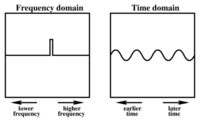 Figure 2
 -
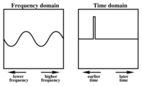 Figure 3
 -
 Figure 4


In a Reed–Solomon code, the frequency domain is divided into two regions as shown in Figure 5: a left (low-frequency) region of length , and a right (high-frequency) region of length . A data word is then embedded into the left region (corresponding to the coefficients of a polynomial of degree at most ), while the right region is filled with zeros. The result is Fourier transformed into the time domain, yielding a code word that is composed only of low frequencies. In the absence of errors, a code word can be decoded by reverse Fourier transforming it back into the frequency domain.

Now consider a code word containing a single error, as shown in red in Figure 6. The effect of this error in the frequency domain is a smooth, single-frequency wave in the right region, called the syndrome of the error. The error location can be determined by determining the frequency of the syndrome signal.
Similarly, if two or more errors are introduced in the code word, the syndrome will be a signal composed of two or more frequencies, as shown in Figure 7. As long as it is possible to determine the frequencies of which the syndrome is composed, it is possible to determine the error locations. Notice that the error locations depend only on the frequencies of these waves, whereas the error magnitudes depend on their amplitudes and phase.
The problem of determining the error locations has therefore been reduced to the problem of finding, given a sequence of values, the smallest set of elementary waves into which these values can be decomposed. It is known from digital signal processing that this problem is equivalent to finding the roots of the minimal polynomial of the sequence, or equivalently, of finding the shortest linear feedback shift register (LFSR) for the sequence. The latter problem can either be solved inefficiently by solving a system of linear equations, or more efficiently by the Berlekamp–Massey algorithm.
-
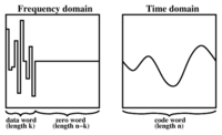 Figure 5
 -
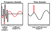 Figure 6
 -
 Figure 7


Decoding beyond the error-correction bound
The Singleton bound states that the minimum distance d of a linear block code of size (n,k) is upper-bounded by n − k + 1. The distance d was usually understood to limit the error-correction capability to ⌊d/2⌋. The Reed–Solomon code achieves this bound with equality, and can thus correct up to ⌊(n − k + 1)/2⌋ errors. However, this error-correction bound is not exact.
In 1999, Madhu Sudan and Venkatesan Guruswami at MIT published “Improved Decoding of Reed–Solomon and Algebraic-Geometry Codes” introducing an algorithm that allowed for the correction of errors beyond half the minimum distance of the code. It applies to Reed–Solomon codes and more generally to algebraic geometric codes. This algorithm produces a list of codewords (it is a list-decoding algorithm) and is based on interpolation and factorization of polynomials over and its extensions.

Soft-decoding
The algebraic decoding methods described above are hard-decision methods, which means that for every symbol a hard decision is made about its value.[7] The advent of LDPC and turbo codes, which employ iterated soft-decision belief propagation decoding methods to achieve error-correction performance close to the theoretical limit, has spurred interest in applying soft-decision decoding to conventional algebraic codes. In 2003, Ralf Koetter and Alexander Vardy presented a polynomial-time soft-decision algebraic list-decoding algorithm for RS codes, which was based upon the work by Sudan and Guruswami.[8]
Applications
Data storage
Reed–Solomon coding is very widely used in mass storage systems to correct the burst errors associated with media defects.
Reed–Solomon coding is a key component of the compact disc. It was the first use of strong error correction coding in a mass-produced consumer product, and DAT and DVD use similar schemes. In the CD, two layers of Reed–Solomon coding separated by a 28-way convolutional interleaver yields a scheme called Cross-Interleaved Reed Solomon Coding (CIRC). The first element of a CIRC decoder is a relatively weak inner (32,28) Reed–Solomon code, shortened from a (255,251) code with 8-bit symbols. This code can correct up to 2 byte errors per 32-byte block. More importantly, it flags as erasures any uncorrectable blocks, i.e., blocks with more than 2 byte errors. The decoded 28-byte blocks, with erasure indications, are then spread by the deinterleaver to different blocks of the (28,24) outer code. Thanks to the deinterleaving, an erased 28-byte block from the inner code becomes a single erased byte in each of 28 outer code blocks. The outer code easily corrects this, since it can handle up to 4 such erasures per block.
The result is a CIRC that can completely correct error bursts up to 4000 bits, or about 2.5 mm on the disc surface. This code is so strong that most CD playback errors are almost certainly caused by tracking errors that cause the laser to jump track, not by uncorrectable error bursts.[9]
Another product which incorporates Reed–Solomon coding is the Nintendo e-Reader. This is a video-game delivery system which uses a two-dimensional barcode printed on trading cards. The cards are scanned using a device which attaches to Nintendo's Game Boy Advance game system.
Reed–Solomon error correction is also used in parchive files which are commonly posted accompanying multimedia files on USENET. The Distributed online storage service Wuala also makes use of Reed–Solomon when breaking up files.
Data transmission
Specialized forms of Reed–Solomon codes, specifically Cauchy-RS and Vandermonde-RS, can be used to overcome the unreliable nature of data transmission over erasure channels. The encoding process assumes a code of RS(N, K) which results in N codewords of length N symbols each storing K symbols of data, being generated, that are then sent over an erasure channel.
Any combination of K codewords received at the other end is enough to reconstruct all of the N codewords. The code rate is generally set to 1/2 unless the channel's erasure likelihood can be adequately modelled and is seen to be less. In conclusion, N is usually 2K, meaning that at least half of all the codewords sent must be received in order to reconstruct all of the codewords sent.
Reed–Solomon codes are also used in xDSL systems and CCSDS's Space Communications Protocol Specifications as a form of forward error correction.
Bar code
Paper bar codes such as PDF-417, PostBar, MaxiCode, Datamatrix, QR Code, and Aztec Code use Reed–Solomon error correction to allow correct reading even if a portion of the bar code is damaged. When the bar code scanner cannot recognize a bar code symbol, it will treat it as an erasure.
Satellite transmission
One significant application of Reed–Solomon coding was to encode the digital pictures sent back by the Voyager space probe.
Voyager introduced Reed–Solomon coding concatenated with convolutional codes, a practice that has since become very widespread in deep space and satellite (e.g., direct digital broadcasting) communications.
Viterbi decoders tend to produce errors in short bursts. Correcting these burst errors is a job best done by short or simplified Reed–Solomon codes.
Modern versions of concatenated Reed–Solomon/Viterbi-decoded convolutional coding were and are used on the Mars Pathfinder, Galileo, Mars Exploration Rover and Cassini missions, where they perform within about 1–1.5 dB of the ultimate limit imposed by the Shannon capacity.
These concatenated codes are now being replaced by more powerful turbo codes where the transmitted data does not need to be decoded immediately.
See also
- BCH code
- Cyclic code
- Chien search
- Berlekamp–Massey algorithm
- Forward error correction
- Berlekamp–Welch algorithm
Notes
- ^ Codes for which each input symbol is from a set of size greater than 2.
- ^ A popular construction is a concatenation of an outer RS code with an inner convolutional code, since the latter delivers errors primarily in bursts.
- ^ There is a slight but usually negligible chance, depending on channel properties, that channel errors turn the message into another valid polynomial.
- ^ Lidl, Rudolf; Pilz, Günter (1999). Applied Abstract Algebra (2nd ed.). Wiley. p. 226.
- ^ See Lin & Costello (1983, p. 171), for example.
- ^ "Kissing Numbers, Sphere Packings, and Some Unexpected Proofs", Notices of the American Mathematical Society, Volume 51, Issue 8, 2004/09. Explains the Delsarte-Goethals-Seidel theorem as used in the context of the error correcting code for compact disc.
- ^ For example, a decoder could associate with each symbol an additional value corresponding to the channel demodulator's confidence in the correctness of the symbol.
- ^ Koetter, Ralf; Vardy, Alexander (2003). "Algebraic soft-decision decoding of Reed–Solomon codes". IEEE Transactions on Information Theory. 49 (11): 2809–2825. doi:10.1109/TIT.2003.819332.
- ^ K.A.S. Immink, Reed–Solomon Codes and the Compact Disc in S.B. Wicker and V.K. Bhargava, Edrs, Reed–Solomon Codes and Their Applications, IEEE Press, 1994.
References
- Cipra, Barry A. (1993), "The Ubiquitous Reed–Solomon Codes", SIAM News, 26 (1)
- Berlekamp, Elwyn R. (1967), Nonbinary BCH decoding, International Symposium on Information Theory, San Remo, Italy
{{citation}}: CS1 maint: location missing publisher (link) - Berlekamp, Elwyn R. (1984) [1968], Algebraic Coding Theory, Laguna Hills, CA: Aegean Park Press, ISBN 0894120638
{{citation}}: Unknown parameter|ed=ignored (help) - Forney, Jr., G. (October 1965), "On Decoding BCH Codes", IEEE Transactions on Information Theory, 11 (4): 549–557, doi:10.1109/TIT.1965.1053825
{{citation}}: CS1 maint: year (link) - Gill, John (unknown), EE387 Notes #7, Handout #28 (PDF), Stanford University, retrieved April 21, 2010
{{citation}}: Check date values in:|year=(help)CS1 maint: year (link) - Hong, Jonathan; Vetterli, Martin (August 1995), "Simple Algorithms for BCH Decoding", IEEE Transactions on Communications, 43 (8): 2324–2333
{{citation}}: CS1 maint: date and year (link) - Koetter, Ralf (2005), Reed–Solomon Codes, MIT Lecture Notes 6.451 (Video)
- Lin, Shu; Costello, Jr., Daniel J. (1983), Error Control Coding: Fundamentals and Applications, New Jersey, NJ: Prentice-Hall, ISBN 0-13-283796-X
- MacWilliams, F. J.; Sloane, N. J. A. (1977), The Theory of Error-Correcting Codes, New York, NY: North-Holland Publishing Company
- Massey, J. L. (1969), "Shift-register synthesis and BCH decoding" (PDF), IEEE Transactions on Information Theory, IT-15 (1): 122–127
- Peterson, Wesley W. (1960), "Encoding and Error Correction Procedures for the Bose-Chaudhuri Codes", IRE Transactions on Information Theory, IT-6, Institute of Radio Engineers: 459–470
- Reed, Irving S.; Chen, Xuemin (1999), Error-Control Coding for Data Networks, Boston, MA: Kluwer Academic Publishers
- Reed, Irving S.; Solomon, Gustave (1960), "Polynomial Codes over Certain Finite Fields", Journal of the Society for Industrial and Applied Mathematics (SIAM), 8 (2): 300–304, doi:10.1137/0108018
- Welch, L. R. (1997), The Original View of Reed–Solomon Codes (PDF), Lecture Notes
External links
- Schifra Open Source C++ Reed–Solomon Codec
- Henry Minsky's RSCode library, Reed–Solomon encoder/decoder
- Open source Verilog Reed-Solomon IP
- A Tutorial on Reed–Solomon Coding for Fault-Tolerance in RAID-like Systems
- Algebraic soft-decoding of Reed–Solomon codes
- Matlab implementation of errors and-erasures Reed–Solomon decoding
- BBC R&D White Paper WHP031
- Geisel, William A. (August 1990), Tutorial on Reed–Solomon Error Correction Coding (PDF), Technical Memorandum, NASA, TM-102162