Lambert W function

"Omega function" redirects here. For the related Wright Omega function, see Wright Omega Function.

The graph of W₀(x) for −1/e ≤ x ≤ 4

In mathematics, the Lambert W function, named after Johann Heinrich Lambert, also called the Omega function or product log, is the inverse function of f(w) = we^w where e^w is the natural exponential function and w is any complex number. The function is denoted here by W. For every complex number z:

$z=W(z)e^{W(z)}.$

Since the function ƒ is not injective, the function W is multivalued (except at 0). If we restrict to real arguments x and demand w real, then the function is defined only for x ≥ −1/e, and is double-valued on (−1/e, 0); the additional constraint w ≥ −1 defines a single-valued function W₀(x), whose graph is shown. We have W₀(0) = 0 and W₀(−1/e) = −1. The alternate branch on [−1/e, 0) with w ≤ −1 is denoted W₋₁(x) and decreases from W₋₁(−1/e) = −1 to W_{−1(0⁻) = −∞.}

The Lambert W function cannot be expressed in terms of elementary functions. It is useful in combinatorics, for instance in the enumeration of trees. It can be used to solve various equations involving exponentials and also occurs in the solution of delay differential equations, such as y'(t) = a y(t − 1).

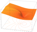
Lambert W function in the complex plane. Note the branch cut running along the negative real axis, ending at −1/e

The canonical reference is by Corless, Gonnet, Hare, Jeffrey and Knuth.

History

Lambert first considered the related Lambert's Transcendental Equation in 1758 which led to a paper by Leonhard Euler in 1783 that discussed the special case of we^w. However the inverse of we^w was first described by Pólya and Szegö in 1925.

Differentiation and integration

By implicit differentiation, one can show that W satisfies the differential equation

$z(1+W){\frac {dW}{dz}}=W\quad \mathrm {for\ } z\neq -1/e,\,$

and hence:

${\frac {dW}{dz}}={\frac {W(z)}{z(1+W(z))}}\quad \mathrm {for\ } z\neq -1/e.\,$

The function W(x), and many expressions involving W(x), can be integrated using the substitution w = W(x), i.e. x = w e^w:

$\int W(x)\,dx=x\left(W(x)-1+{\frac {1}{W(x)}}\right)+C.$

Taylor series

The Taylor series of W₀ around 0 can be found using the Lagrange inversion theorem and is given by

$W_{0}(x)=\sum _{n=1}^{\infty }{\frac {(-n)^{n-1}}{n!}}\ x^{n}=x-x^{2}+{\frac {3}{2}}x^{3}-{\frac {8}{3}}x^{4}+{\frac {125}{24}}x^{5}-\cdots$

The radius of convergence is 1/e, as may be seen by the ratio test. The function defined by this series can be extended to a holomorphic function defined on all complex numbers with a branch cut along the interval (−∞, −1/e]; this holomorphic function defines the principal branch of the Lambert W function.

Special values

$W\left(-{\tfrac {1}{2}}\pi \right)={\tfrac {1}{2}}\pi \mathrm {i}$

$W\left(-{\tfrac {1}{2}}\ln 2\right)=-\ln 2$

$W\left(-{\tfrac {1}{a}}\ln a\right)=-\ln a\dots {\tfrac {1}{e}}\leq a\leq e$

$W\left(-{1 \over e}\right)=-1$

$W(0)=0\,$

$W(1)=\Omega \approx 0.56714329\dots \,$ (the Omega constant)

$W(e)=1\,$

$W(-1)=-0.31813\dots -1.33723\dots {\mathrm {i} }\,$

Applications

The Lambert function has been applied to solve problems in the analysis of algorithms, the spread of disease, quantum physics, ideal diodes and transistors, black holes, the kinetics of pigment regeneration in the human eye, dynamical systems containing delays, and in many other areas.

Many equations involving exponentials can be solved using the W function. The general strategy is to move all instances of the unknown to one side of the equation and make it look like Y = Xe^X at which point the W function provides the solution.

In other words :

$Y=Xe^{X}\;\Longleftrightarrow \;X=W(Y)$

Examples

Example 1

$2^{t}=5t\,$

$\Rightarrow 1={\frac {5t}{2^{t}}}\,$

$\Rightarrow 1=5t\,e^{-t\ln 2}\,$

$\Rightarrow {\frac {1}{5}}=t\,e^{-t\ln 2}\,$

$\Rightarrow {\frac {-\,\ln 2}{5}}=(-\,t\,\ln 2)\,e^{(-t\ln 2)}\,$

$\Rightarrow -t\ln 2=W\left({\frac {-\ln 2}{5}}\right)\,$

$\Rightarrow t={\frac {-W\left({\frac {-\ln 2}{5}}\right)}{\ln 2}}\,$

More generally, the equation

$~p^{ax+b}=cx+d$

where

$p>0\land c,d\neq 0$

can be transformed via the substitution

$-t=ax+{\frac {ad}{c}}$

into

$tp^{t}=R=-{\frac {a}{c}}p^{b-{\frac {ad}{c}}}$

giving

$t={\frac {W(R\ln p)}{\ln p}}$

which yields the final solution

$x=-{\frac {W(-{\frac {a\ln p}{c}}\,p^{b-{\frac {ad}{c}}})}{a\ln p}}-{\frac {d}{c}}$

Example 2

Similar techniques show that

$x^{x}=z\,,$

has solution

$x={\frac {\ln(z)}{W(\ln z)}}\,,$

or, equivalently,

$x=\exp \left(W(\ln(z))\right).$

Example 3

Whenever the complex infinite exponential tetration

$z^{z^{z^{\cdot ^{\cdot ^{\cdot }}}}}\!$

converges, the Lambert W function provides the actual limit value as

$c={\frac {W(-\ln(z))}{-\ln(z)}}$

where ln(z) denotes the principal branch of the complex log function.

Example 4

Solutions for

$x\log _{b}\left(x\right)=a$

have the form

$x={\frac {a\ln(b)}{W(a\ln(b))}}$

Example 5

The solution for the current in a series diode/resistor circuit can also be written in terms of the Lambert W. See diode modeling.

Example 6

The delay differential equation

${\dot {y}}(t)=ay(t-1)$

has characteristic equation $\lambda =ae^{-\lambda }$, leading to $\lambda =W_{k}(a)$ and $y(t)=e^{W_{k}(a)t}$, where $k$ is the branch index. If $a$ is real, only $W_{0}(a)$ need be considered.

Generalizations

The standard Lambert W function expresses exact solutions to transcendental algebraic equations (in x) of the form:

$e^{-cx}=a_{o}(x-r)~~\quad \qquad \qquad \qquad \qquad (1)$

where a₀, c and r are real constants. The solution is $x=r+{\frac {1}{c}}W({\frac {ce^{-cr}}{a_{o}}})\,$. Generalizations of the Lambert W function include:

• An application to general relativity and quantum mechanics in lower dimensions, in fact a previously unknown link between these two areas, as shown in the Journal of Classical and Quantum Gravity where the right-hand-side of (1) is now a quadratic polynomial in x:

$e^{-cx}=a_{o}(x-r_{1})(x-r_{2})~~\qquad \qquad (2)$

and where r₁ and r₂ are real distinct constants, the roots of the quadratic polynomial. Here, the solution is a function has a single argument x but the terms like r_i and a_o are parameters of that function. In this respect, the generalization resembles the hypergeometric function and the Meijer G-function but it belongs to a different class of functions. When r₁ = r₂, both sides of (2) can be factored and reduced to (1) and thus the solution reduces to that of the standard W function. Eq. (2) expresses the equation governing the dilaton field, from which is derived the metric of the lineal two-body gravity problem in 1+1 dimensions (one spatial dimension and one time dimension) for the case of unequal (rest) masses, as well as, the eigenenergies of the quantum-mechanical double-well Dirac delta function model for unequal charges in one dimension.

• Analytical solutions of the eigenenergies of a special case of the quantum mechanical three-body problem, namely the (three-dimensional) hydrogen molecule-ion. Here the right-hand-side of (1) (or (2)) is now a ratio of infinite order polynomials in x:

$e^{-cx}=a_{o}{\frac {\prod _{i=1}^{\infty }(x-r_{i})}{\prod _{i=1}^{\infty }(x-s_{i})}}\qquad \qquad \qquad (3)$

where r_i and s_i are distinct real constants and x is a function of the eigenenergy and the internuclear distance R. Eq. (3) with its specialized cases expressed in (1) and (2) is related to a large class of delay differential equations.

Applications of the Lambert "W" function in fundamental physical problems are not exhausted even for the standard case expressed in (1) as seen recently in the area of atomic, molecular, and optical physics.

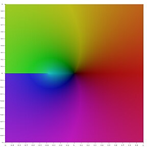
Plots

• Plots of the LambertW function on the complex plane
• 
  z = Re(W₀(x + i y))
• 
  z = Im(W₀(x + i y))
• 
• 

Numerical evaluation

Iterative algorithm

The W function may be approximated using Newton's method, with successive approximations to $w=W(z)$ (so $z=we^{w}$) being

$w_{j+1}=w_{j}-{\frac {w_{j}e^{w_{j}}-z}{e^{w_{j}}+w_{j}e^{w_{j}}}}.$

The W function may also be approximated using Halley's method,

$w_{j+1}=w_{j}-{\frac {w_{j}e^{w_{j}}-z}{e^{w_{j}}(w_{j}+1)-{\frac {(w_{j}+2)(w_{j}e^{w_{j}}-z)}{2w_{j}+2}}}}$

given in Corless et al. to compute W. Together with the evaluation error estimate given in Chapeau-Blondeau and Monir, the following Python code, which computes the principal branch for $x>-1/e$, implements this. Note: the success of this code is closely dependent on the initial estimates (e.g., w = 0).

from math import e
 
def lambertW(x, prec=1E-12, maxiters=100):
    w = 0    

    for i in range(maxiters):
        we = w * e**w
        w1e = (w + 1) * e**w

        if prec > abs((x - we) / w1e):
            return w

        w -= (we - x) / (w1e - (w + 2) * (we - x) / (2*w + 2))
        
    raise ValueError("W doesn't converge fast enough for abs(z) = %f" % abs(x))

Approximation

The following closed form approximation for values of x greater than or equal to zero may be used by itself when less accuracy is needed, or to give an excellent initial estimate to the above code, which then may need only a few iterations:

double
desy_lambert_W(double x) {
      double  lx1;
      if (x <= 500.0) {
              lx1 = ln(x + 1.0);
              return 0.665 * (1 + 0.0195 * lx1) * lx1 + 0.04;
      }
      return ln(x - 4.0) - (1.0 - 1.0/ln(x)) * ln(ln(x));
}

(from http://www.desy.de/~t00fri/qcdins/texhtml/lambertw/)

See also

• Lambert's trinomial equation

References and external links

• MathWorld - Lambert W-Function
• Lambert function from Wolfram's function site.
• Computing the Lambert Wfunction
• Corless et al. Notes about Lambert W research
• Corless et al. "On the Lambert W function" Adv. Computational Maths. 5, 329 - 359 (1996) (PDF)
• Chapeau-Blondeau, F. and Monir, A: "Evaluation of the Lambert W Function and Application to Generation of Generalized Gaussian Noise With Exponent 1/2", IEEE Trans. Signal Processing, 50(9), 2002
• Francis et al. "Quantitative General Theory for Periodic Breathing" Circulation 102 (18): 2214. (2000). Use of Lambert function to solve delay-differential dynamics in human disease.
• Extreme Mathematics. Monographs on the Lambert W function, its numerical approximation and generalizations for W-like inverses of transcendental forms with repeated exponential towers.