Mathematical term
Function
S
(
q
)
=
∑
n
=
1
∞
q
n
1
−
q
n
{\textstyle S(q)=\sum _{n=1}^{\infty }{\frac {q^{n}}{1-q^{n}}}}
, represented as a Matplotlib plot, using a version of the domain coloring method[ 1]
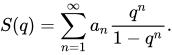
In mathematics , a Lambert series , named for Johann Heinrich Lambert , is a series taking the form
S
(
q
)
=
∑
n
=
1
∞
a
n
q
n
1
−
q
n
.

{\displaystyle S(q)=\sum _{n=1}^{\infty }a_{n}{\frac {q^{n}}{1-q^{n}}}.}
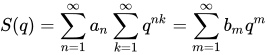
It can be resummed formally by expanding the denominator:
S
(
q
)
=
∑
n
=
1
∞
a
n
∑
k
=
1
∞
q
n
k
=
∑
m
=
1
∞
b
m
q
m
{\displaystyle S(q)=\sum _{n=1}^{\infty }a_{n}\sum _{k=1}^{\infty }q^{nk}=\sum _{m=1}^{\infty }b_{m}q^{m}}
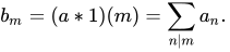
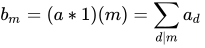
where the coefficients of the new series are given by the Dirichlet convolution of a n with the constant function 1(n ) = 1:
b
m
=
(
a
∗
1
)
(
m
)
=
∑
n
∣
m
a
n
.
{\displaystyle b_{m}=(a*1)(m)=\sum _{n\mid m}a_{n}.\,}
This series may be inverted by means of the Möbius inversion formula , and is an example of a Möbius transform .
Since this last sum is a typical number-theoretic sum, almost any natural multiplicative function will be exactly summable when used in a Lambert series. Thus, for example, one has
∑
n
=
1
∞
q
n
σ
0
(
n
)
=
∑
n
=
1
∞
q
n
1
−
q
n
{\displaystyle \sum _{n=1}^{\infty }q^{n}\sigma _{0}(n)=\sum _{n=1}^{\infty }{\frac {q^{n}}{1-q^{n}}}}
where
σ
0
(
n
)
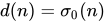
=
d
(
n
)
{\displaystyle \sigma _{0}(n)=d(n)}
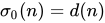
is the number of positive divisors of the number n .
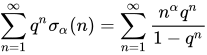
For the higher order sum-of-divisor functions , one has
∑
n
=
1
∞
q
n
σ
α
(
n
)
=
∑
n
=
1
∞
n
α
q
n
1
−
q
n
=
∑
n
=
1
∞
Li
−
α
(
q
n
)
{\displaystyle \sum _{n=1}^{\infty }q^{n}\sigma _{\alpha }(n)=\sum _{n=1}^{\infty }{\frac {n^{\alpha }q^{n}}{1-q^{n}}}=\sum _{n=1}^{\infty }\operatorname {Li} _{-\alpha }(q^{n})}
where
α
{\displaystyle \alpha }
is any complex number ,
Li
{\displaystyle \operatorname {Li} }
is the polylogarithm , and
σ
α
(
n
)
=
(
Id
α
∗
1
)
(
n
)
=
∑
d
∣
n
d
α
{\displaystyle \sigma _{\alpha }(n)=({\textrm {Id}}_{\alpha }*1)(n)=\sum _{d\mid n}d^{\alpha }\,}
is the divisor function. In particular, for
α
=
1
{\displaystyle \alpha =1}
, the Lambert series one gets is
q
F
′
(
q
)
F
(
q
)
{\displaystyle q{\frac {F'(q)}{F(q)}}}
which is (up to the factor of
q
{\displaystyle q}
) the logarithmic derivative of the usual generating function for partition numbers
F
(
q
)
:=
1
ϕ
(
q
)
=
∑
k
=
0
∞
p
(
k
)
q
k
=
∏
n
=
1
∞
1
1
−
q
n
.
{\displaystyle F(q):={\frac {1}{\phi (q)}}=\sum _{k=0}^{\infty }p(k)q^{k}=\prod _{n=1}^{\infty }{\frac {1}{1-q^{n}}}.}
Additional Lambert series related to the previous identity include those for the variants of the
Möbius function given below
μ
(
n
)
{\displaystyle \mu (n)}
[ 2]
∑
n
=
1
∞
μ
(
n
)
q
n
1
−
q
n
=
q
.
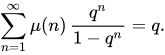
{\displaystyle \sum _{n=1}^{\infty }\mu (n)\,{\frac {q^{n}}{1-q^{n}}}=q.}
Related Lambert series over the Möbius function include the following identities for any
prime
α
∈
Z
+
{\displaystyle \alpha \in \mathbb {Z} ^{+}}
:
∑
n
≥
1
μ
(
n
)
q
n
1
+
q
n
=
q
−
2
q
2
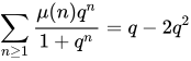
{\displaystyle \sum _{n\geq 1}{\frac {\mu (n)q^{n}}{1+q^{n}}}=q-2q^{2}}
∑
n
≥
1
μ
(
α
n
)
q
n
1
−
q
n
=
−
∑
n
≥
0
q
α
n
.
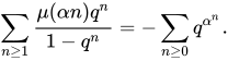
{\displaystyle \sum _{n\geq 1}{\frac {\mu (\alpha n)q^{n}}{1-q^{n}}}=-\sum _{n\geq 0}q^{\alpha ^{n}}.}
[citation needed ]
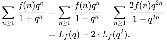
The proof of the first identity above follows from a multi-section (or bisection) identity of these
Lambert series generating functions in the following form where we denote
L
f
(
q
)
:=
q
{\displaystyle L_{f}(q):=q}
to be the Lambert series generating function of the arithmetic function f :
∑
n
≥
1
f
(
n
)
q
n
1
+
q
n
=
∑
n
≥
1
f
(
n
)
q
n
1
−
q
n
−
∑
n
≥
1
2
f
(
n
)
q
2
n
1
−
q
2
n
=
L
f
(
q
)
−
2
⋅
L
f
(
q
2
)
.
{\displaystyle {\begin{aligned}\sum _{n\geq 1}{\frac {f(n)q^{n}}{1+q^{n}}}&=\sum _{n\geq 1}{\frac {f(n)q^{n}}{1-q^{n}}}-\sum _{n\geq 1}{\frac {2f(n)q^{2n}}{1-q^{2n}}}\\&=L_{f}(q)-2\cdot L_{f}(q^{2}).\end{aligned}}}
For Euler's totient function
φ
(
n
)
{\displaystyle \varphi (n)}
:
∑
n
=
1
∞
φ
(
n
)
q
n
1
−
q
n
=
q
(
1
−
q
)
2
.
{\displaystyle \sum _{n=1}^{\infty }\varphi (n)\,{\frac {q^{n}}{1-q^{n}}}={\frac {q}{(1-q)^{2}}}.}
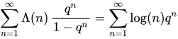
For Von Mangoldt function
Λ
(
n
)
{\displaystyle \Lambda (n)}
:
∑
n
=
1
∞
Λ
(
n
)
q
n
1
−
q
n
=
∑
n
=
1
∞
log
(
n
)
q
n
{\displaystyle \sum _{n=1}^{\infty }\Lambda (n)\,{\frac {q^{n}}{1-q^{n}}}=\sum _{n=1}^{\infty }\log(n)q^{n}}
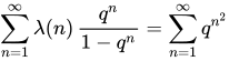
For Liouville's function
λ
(
n
)
{\displaystyle \lambda (n)}
:
∑
n
=
1
∞
λ
(
n
)
q
n
1
−
q
n
=
∑
n
=
1
∞
q
n
2
{\displaystyle \sum _{n=1}^{\infty }\lambda (n)\,{\frac {q^{n}}{1-q^{n}}}=\sum _{n=1}^{\infty }q^{n^{2}}}
with the sum on the right similar to the Ramanujan theta function , or Jacobi theta function
ϑ
3
(
q
)
{\displaystyle \vartheta _{3}(q)}
. Note that Lambert series in which the a n are trigonometric functions , for example, a n = sin(2n x ), can be evaluated by various combinations of the logarithmic derivatives of Jacobi theta functions .
Generally speaking, we can extend the previous generating function expansion by letting
χ
m
(
n
)
{\displaystyle \chi _{m}(n)}
denote the characteristic function of the
m
t
h
{\displaystyle m^{th}}
powers,
n
=
k
m
∈
Z
+
{\displaystyle n=k^{m}\in \mathbb {Z} ^{+}}
, for positive natural numbers
m
>
2
{\displaystyle m>2}
and defining the generalized m -Liouville lambda function to be the arithmetic function satisfying
χ
m
(
n
)
:=
(
1
∗
λ
m
)
(
n
)
{\displaystyle \chi _{m}(n):=(1\ast \lambda _{m})(n)}
. This definition of
λ
m
(
n
)
{\displaystyle \lambda _{m}(n)}
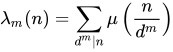
clearly implies that
λ
m
(
n
)
=
∑
d
m
|
n
μ
(
n
d
m
)
{\displaystyle \lambda _{m}(n)=\sum _{d^{m}|n}\mu \left({\frac {n}{d^{m}}}\right)}
, which in turn shows that
∑
n
≥
1
λ
m
(
n
)
q
n
1
−
q
n
=
∑
n
≥
1
q
n
m
,
for
m
≥
2.
{\displaystyle \sum _{n\geq 1}{\frac {\lambda _{m}(n)q^{n}}{1-q^{n}}}=\sum _{n\geq 1}q^{n^{m}},\ {\text{ for }}m\geq 2.}
We also have a slightly more generalized Lambert series expansion generating the sum of squares function
r
2
(
n
)
{\displaystyle r_{2}(n)}
in the form of
[ 3]
∑
n
=
1
∞
4
⋅
(
−
1
)
n
+
1
q
2
n
+
1
1
−
q
2
n
+
1
=
∑
m
=
1
∞
r
2
(
m
)
q
m
.
{\displaystyle \sum _{n=1}^{\infty }{\frac {4\cdot (-1)^{n+1}q^{2n+1}}{1-q^{2n+1}}}=\sum _{m=1}^{\infty }r_{2}(m)q^{m}.}
In general, if we write the Lambert series over
f
(
n
)
{\displaystyle f(n)}
which generates the arithmetic functions
g
(
m
)
=
(
f
∗
1
)
(
m
)
{\displaystyle g(m)=(f\ast 1)(m)}
, the next pairs of functions correspond to other well-known convolutions expressed by their Lambert series generating functions in the forms of
(
f
,
g
)
=
(
μ
,
ε
)
,
(
φ
,
Id
1
)
,
(
λ
,
χ
sq
)
,
(
Λ
,
log
)
,
(
|
μ
|
,
2
ω
)
,
(
J
t
,
Id
t
)
,
(
d
3
,
(
d
∗
1
)
2
)
,
{\displaystyle (f,g)=(\mu ,\varepsilon ),(\varphi ,\operatorname {Id} _{1}),(\lambda ,\chi _{\operatorname {sq} }),(\Lambda ,\log ),(|\mu |,2^{\omega }),(J_{t},\operatorname {Id} _{t}),(d^{3},(d\ast 1)^{2}),}
where
ε
(
n
)
=
δ
n
,
1
{\displaystyle \varepsilon (n)=\delta _{n,1}}
is the multiplicative identity for Dirichlet convolutions ,
Id
k
(
n
)
=
n
k
{\displaystyle \operatorname {Id} _{k}(n)=n^{k}}
is the identity function for
k
t
h
{\displaystyle k^{th}}
powers,
χ
sq
{\displaystyle \chi _{\operatorname {sq} }}
denotes the characteristic function for the squares,
ω
(
n
)
{\displaystyle \omega (n)}
which counts the number of distinct prime factors of
n
{\displaystyle n}
(see prime omega function ),
J
t
{\displaystyle J_{t}}
is Jordan's totient function , and
d
(
n
)
=
σ
0
(
n
)
{\displaystyle d(n)=\sigma _{0}(n)}
is the divisor function (see Dirichlet convolutions ).
The conventional use of the letter q in the summations is a historical usage, referring to its origins in the theory of elliptic curves and theta functions, as the nome .
Substituting
q
=
e
−
z
{\displaystyle q=e^{-z}}
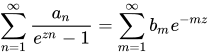
one obtains another common form for the series, as
∑
n
=
1
∞
a
n
e
z
n
−
1
=
∑
m
=
1
∞
b
m
e
−
m
z
{\displaystyle \sum _{n=1}^{\infty }{\frac {a_{n}}{e^{zn}-1}}=\sum _{m=1}^{\infty }b_{m}e^{-mz}}
where
b
m
=
(
a
∗
1
)
(
m
)
=
∑
d
∣
m
a
d
{\displaystyle b_{m}=(a*1)(m)=\sum _{d\mid m}a_{d}\,}
as before. Examples of Lambert series in this form, with
z
=
2
π
{\displaystyle z=2\pi }
, occur in expressions for the Riemann zeta function for odd integer values; see Zeta constants for details.
In the literature we find Lambert series applied to a wide variety of sums. For example, since
q
n
/
(
1
−
q
n
)
=
L
i
0
(
q
n
)
{\displaystyle q^{n}/(1-q^{n})=\mathrm {Li} _{0}(q^{n})}
is a polylogarithm function, we may refer to any sum of the form
∑
n
=
1
∞
ξ
n
L
i
u
(
α
q
n
)
n
s
=
∑
n
=
1
∞
α
n
L
i
s
(
ξ
q
n
)
n
u
{\displaystyle \sum _{n=1}^{\infty }{\frac {\xi ^{n}\,\mathrm {Li} _{u}(\alpha q^{n})}{n^{s}}}=\sum _{n=1}^{\infty }{\frac {\alpha ^{n}\,\mathrm {Li} _{s}(\xi q^{n})}{n^{u}}}}
as a Lambert series, assuming that the parameters are suitably restricted. Thus
12
(
∑
n
=
1
∞
n
2
L
i
−
1
(
q
n
)
)
2
=
∑
n
=
1
∞
n
2
L
i
−
5
(
q
n
)
−
∑
n
=
1
∞
n
4
L
i
−
3
(
q
n
)
,
{\displaystyle 12\left(\sum _{n=1}^{\infty }n^{2}\,\mathrm {Li} _{-1}(q^{n})\right)^{\!2}=\sum _{n=1}^{\infty }n^{2}\,\mathrm {Li} _{-5}(q^{n})-\sum _{n=1}^{\infty }n^{4}\,\mathrm {Li} _{-3}(q^{n}),}
which holds for all complex q not on the unit circle , would be considered a Lambert series identity. This identity follows in a straightforward fashion from some identities published by the Indian mathematician S. Ramanujan . A very thorough exploration of Ramanujan's works can be found in the works by Bruce Berndt .
Factorization theorems [ edit ]
A somewhat newer construction recently published over 2017–2018 relates to so-termed Lambert series factorization theorems of the form[ 4]
∑
n
≥
1
a
n
q
n
1
±
q
n
=
1
(
∓
q
;
q
)
∞
∑
n
≥
1
(
(
s
o
(
n
,
k
)
±
s
e
(
n
,
k
)
)
a
k
)
q
n
,
{\displaystyle \sum _{n\geq 1}{\frac {a_{n}q^{n}}{1\pm q^{n}}}={\frac {1}{(\mp q;q)_{\infty }}}\sum _{n\geq 1}\left((s_{o}(n,k)\pm s_{e}(n,k))a_{k}\right)q^{n},}
where
s
o
(
n
,
k
)
±
s
e
(
n
,
k
)
=
[
q
n
]
(
∓
q
;
q
)
∞
q
k
1
±
q
k
{\displaystyle s_{o}(n,k)\pm s_{e}(n,k)=[q^{n}](\mp q;q)_{\infty }{\frac {q^{k}}{1\pm q^{k}}}}
is the respective sum or difference of the
restricted partition functions
s
e
/
o
(
n
,
k
)
{\displaystyle s_{e/o}(n,k)}
which denote the number of
k
{\displaystyle k}
's in all partitions of
n
{\displaystyle n}
into an even (respectively, odd ) number of distinct parts. Let
s
n
,
k
:=
s
e
(
n
,
k
)
−
s
o
(
n
,
k
)
=
[
q
n
]
(
q
;
q
)
∞
q
k
1
−
q
k
{\displaystyle s_{n,k}:=s_{e}(n,k)-s_{o}(n,k)=[q^{n}](q;q)_{\infty }{\frac {q^{k}}{1-q^{k}}}}
denote the invertible lower triangular sequence whose first few values are shown in the table below.
n \ k
1
2
3
4
5
6
7
8
1
1
0
0
0
0
0
0
0
2
0
1
0
0
0
0
0
0
3
-1
-1
1
0
0
0
0
0
4
-1
0
-1
1
0
0
0
0
5
-1
-1
-1
-1
1
0
0
0
6
0
0
1
-1
-1
1
0
0
7
0
0
-1
0
-1
-1
1
0
8
1
0
0
1
0
-1
-1
1
Another characteristic form of the Lambert series factorization theorem expansions is given by[ 5]
L
f
(
q
)
:=
∑
n
≥
1
f
(
n
)
q
n
1
−
q
n
=
1
(
q
;
q
)
∞
∑
n
≥
1
(
s
n
,
k
f
(
k
)
)
q
n
,
{\displaystyle L_{f}(q):=\sum _{n\geq 1}{\frac {f(n)q^{n}}{1-q^{n}}}={\frac {1}{(q;q)_{\infty }}}\sum _{n\geq 1}\left(s_{n,k}f(k)\right)q^{n},}
where
(
q
;
q
)
∞
{\displaystyle (q;q)_{\infty }}
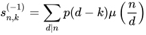
is the (infinite) q-Pochhammer symbol . The invertible matrix products on the right-hand-side of the previous equation correspond to inverse matrix products whose lower triangular entries are given in terms of the partition function and the Möbius function by the divisor sums
s
n
,
k
(
−
1
)
=
∑
d
|
n
p
(
d
−
k
)
μ
(
n
d
)
{\displaystyle s_{n,k}^{(-1)}=\sum _{d|n}p(d-k)\mu \left({\frac {n}{d}}\right)}
The next table lists the first several rows of these corresponding inverse matrices.[ 6]
n \ k
1
2
3
4
5
6
7
8
1
1
0
0
0
0
0
0
0
2
0
1
0
0
0
0
0
0
3
1
1
1
0
0
0
0
0
4
2
1
1
1
0
0
0
0
5
4
3
2
1
1
0
0
0
6
5
3
2
2
1
1
0
0
7
10
7
5
3
2
1
1
0
8
12
9
6
4
3
2
1
1
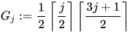
We let
G
j
:=
1
2
⌈
j
2
⌉
⌈
3
j
+
1
2
⌉
{\displaystyle G_{j}:={\frac {1}{2}}\left\lceil {\frac {j}{2}}\right\rceil \left\lceil {\frac {3j+1}{2}}\right\rceil }
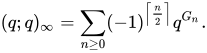
denote the sequence of interleaved pentagonal numbers , i.e., so that the pentagonal number theorem is expanded in the form of
(
q
;
q
)
∞
=
∑
n
≥
0
(
−
1
)
⌈
n
2
⌉
q
G
n
.
{\displaystyle (q;q)_{\infty }=\sum _{n\geq 0}(-1)^{\left\lceil {\frac {n}{2}}\right\rceil }q^{G_{n}}.}
Then for any Lambert series
L
f
(
q
)
{\displaystyle L_{f}(q)}
generating the sequence of
g
(
n
)
=
(
f
∗
1
)
(
n
)
{\displaystyle g(n)=(f\ast 1)(n)}
, we have the corresponding inversion relation of the factorization theorem expanded above given by[ 7]
f
(
n
)
=
∑
k
=
1
n
∑
d
|
n
p
(
d
−
k
)
μ
(
n
/
d
)
×
∑
j
:
k
−
G
j
>
0
(
−
1
)
⌈
j
2
⌉
b
(
k
−
G
j
)
.
{\displaystyle f(n)=\sum _{k=1}^{n}\sum _{d|n}p(d-k)\mu (n/d)\times \sum _{j:k-G_{j}>0}(-1)^{\left\lceil {\frac {j}{2}}\right\rceil }b(k-G_{j}).}
This work on Lambert series factorization theorems is extended in[ 8] to more general expansions of the form
∑
n
≥
1
a
n
q
n
1
−
q
n
=
1
C
(
q
)
∑
n
≥
1
(
∑
k
=
1
n
s
n
,
k
(
γ
)
a
~
k
(
γ
)
)
q
n
,
{\displaystyle \sum _{n\geq 1}{\frac {a_{n}q^{n}}{1-q^{n}}}={\frac {1}{C(q)}}\sum _{n\geq 1}\left(\sum _{k=1}^{n}s_{n,k}(\gamma ){\widetilde {a}}_{k}(\gamma )\right)q^{n},}
where
C
(
q
)
{\displaystyle C(q)}
is any (partition-related) reciprocal generating function,
γ
(
n
)
{\displaystyle \gamma (n)}
is any arithmetic function , and where the
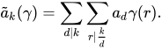
modified coefficients are expanded by
a
~
k
(
γ
)
=
∑
d
|
k
∑
r
|
k
d
a
d
γ
(
r
)
.
{\displaystyle {\widetilde {a}}_{k}(\gamma )=\sum _{d|k}\sum _{r|{\frac {k}{d}}}a_{d}\gamma (r).}
The corresponding inverse matrices in the above expansion satisfy
s
n
,
k
(
−
1
)
(
γ
)
=
∑
d
|
n
[
q
d
−
k
]
1
C
(
q
)
γ
(
n
d
)
,
{\displaystyle s_{n,k}^{(-1)}(\gamma )=\sum _{d|n}[q^{d-k}]{\frac {1}{C(q)}}\gamma \left({\frac {n}{d}}\right),}
so that as in the first variant of the Lambert factorization theorem above we obtain an inversion relation for the right-hand-side coefficients of the form
a
~
k
(
γ
)
=
∑
k
=
1
n
s
n
,
k
(
−
1
)
(
γ
)
×
[
q
k
]
(
∑
d
=
1
k
a
d
q
d
1
−
q
d
C
(
q
)
)
.
{\displaystyle {\widetilde {a}}_{k}(\gamma )=\sum _{k=1}^{n}s_{n,k}^{(-1)}(\gamma )\times [q^{k}]\left(\sum _{d=1}^{k}{\frac {a_{d}q^{d}}{1-q^{d}}}C(q)\right).}
Recurrence relations [ edit ]
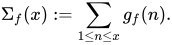
Within this section we define the following functions for natural numbers
n
,
x
≥
1
{\displaystyle n,x\geq 1}
:
g
f
(
n
)
:=
(
f
∗
1
)
(
n
)
,
{\displaystyle g_{f}(n):=(f\ast 1)(n),}
Σ
f
(
x
)
:=
∑
1
≤
n
≤
x
g
f
(
n
)
.
{\displaystyle \Sigma _{f}(x):=\sum _{1\leq n\leq x}g_{f}(n).}
We also adopt the notation from the previous section that
s
n
,
k
=
[
q
n
]
(
q
;
q
)
∞
q
k
1
−
q
k
,
{\displaystyle s_{n,k}=[q^{n}](q;q)_{\infty }{\frac {q^{k}}{1-q^{k}}},}
where
(
q
;
q
)
∞
{\displaystyle (q;q)_{\infty }}
is the infinite q-Pochhammer symbol . Then we have the following recurrence relations for involving these functions and the pentagonal numbers proved in:[ 7]
g
f
(
n
+
1
)
=
∑
b
=
±
1
∑
k
=
1
⌊
24
n
+
1
−
b
6
⌋
(
−
1
)
k
+
1
g
f
(
n
+
1
−
k
(
3
k
+
b
)
2
)
+
∑
k
=
1
n
+
1
s
n
+
1
,
k
f
(
k
)
,
{\displaystyle g_{f}(n+1)=\sum _{b=\pm 1}\sum _{k=1}^{\left\lfloor {\frac {{\sqrt {24n+1}}-b}{6}}\right\rfloor }(-1)^{k+1}g_{f}\left(n+1-{\frac {k(3k+b)}{2}}\right)+\sum _{k=1}^{n+1}s_{n+1,k}f(k),}
Σ
f
(
x
+
1
)
=
∑
b
=
±
1
∑
k
=
1
⌊
24
x
+
1
−
b
6
⌋
(
−
1
)
k
+
1
Σ
f
(
n
+
1
−
k
(
3
k
+
b
)
2
)
+
∑
n
=
0
x
∑
k
=
1
n
+
1
s
n
+
1
,
k
f
(
k
)
.
{\displaystyle \Sigma _{f}(x+1)=\sum _{b=\pm 1}\sum _{k=1}^{\left\lfloor {\frac {{\sqrt {24x+1}}-b}{6}}\right\rfloor }(-1)^{k+1}\Sigma _{f}\left(n+1-{\frac {k(3k+b)}{2}}\right)+\sum _{n=0}^{x}\sum _{k=1}^{n+1}s_{n+1,k}f(k).}
Derivatives of a Lambert series can be obtained by differentiation of the series termwise with respect to
q
{\displaystyle q}
. We have the following identities for the termwise
s
t
h
{\displaystyle s^{th}}
derivatives of a Lambert series for any
s
≥
1
{\displaystyle s\geq 1}
[ 9] [ 10]
q
s
⋅
D
(
s
)
[
q
i
1
−
q
i
]
=
∑
m
=
0
s
∑
k
=
0
m
[
s
m
]
{
m
k
}
(
−
1
)
s
−
k
k
!
i
m
(
1
−
q
i
)
k
+
1
{\displaystyle q^{s}\cdot D^{(s)}\left[{\frac {q^{i}}{1-q^{i}}}\right]=\sum _{m=0}^{s}\sum _{k=0}^{m}\left[{\begin{matrix}s\\m\end{matrix}}\right]\left\{{\begin{matrix}m\\k\end{matrix}}\right\}{\frac {(-1)^{s-k}k!i^{m}}{(1-q^{i})^{k+1}}}}
q
s
⋅
D
(
s
)
[
q
i
1
−
q
i
]
=
∑
r
=
0
s
[
∑
m
=
0
s
∑
k
=
0
m
[
s
m
]
{
m
k
}
(
s
−
k
r
)
(
−
1
)
s
−
k
−
r
k
!
i
m
(
1
−
q
i
)
k
+
1
]
q
(
r
+
1
)
i
,
{\displaystyle q^{s}\cdot D^{(s)}\left[{\frac {q^{i}}{1-q^{i}}}\right]=\sum _{r=0}^{s}\left[\sum _{m=0}^{s}\sum _{k=0}^{m}\left[{\begin{matrix}s\\m\end{matrix}}\right]\left\{{\begin{matrix}m\\k\end{matrix}}\right\}{\binom {s-k}{r}}{\frac {(-1)^{s-k-r}k!i^{m}}{(1-q^{i})^{k+1}}}\right]q^{(r+1)i},}
where the bracketed triangular coefficients in the previous equations denote the Stirling numbers of the first and second kinds .
We also have the next identity for extracting the individual coefficients of the terms implicit to the previous expansions given in the form of
[
q
n
]
(
∑
i
≥
t
a
i
q
m
i
(
1
−
q
i
)
k
+
1
)
=
∑
d
|
n
t
≤
d
≤
⌊
n
m
⌋
(
n
d
−
m
+
k
k
)
a
d
.
{\displaystyle [q^{n}]\left(\sum _{i\geq t}{\frac {a_{i}q^{mi}}{(1-q^{i})^{k+1}}}\right)=\sum _{\begin{matrix}d|n\\t\leq d\leq \left\lfloor {\frac {n}{m}}\right\rfloor \end{matrix}}{\binom {{\frac {n}{d}}-m+k}{k}}a_{d}.}
Now if we define the functions
A
t
(
n
)
{\displaystyle A_{t}(n)}
for any
n
,
t
≥
1
{\displaystyle n,t\geq 1}
by
A
t
(
n
)
:=
∑
0
≤
k
≤
m
≤
t
0
≤
r
≤
t
∑
d
|
n
[
t
m
]
{
m
k
}
(
t
−
k
r
)
(
n
d
−
1
−
r
+
k
k
)
(
−
1
)
t
−
k
−
r
k
!
d
m
⋅
a
d
⋅
[
t
≤
d
≤
⌊
n
r
+
1
⌋
]
δ
,
{\displaystyle A_{t}(n):=\sum _{\begin{matrix}0\leq k\leq m\leq t\\0\leq r\leq t\end{matrix}}\sum _{d|n}\left[{\begin{matrix}t\\m\end{matrix}}\right]\left\{{\begin{matrix}m\\k\end{matrix}}\right\}{\binom {t-k}{r}}{\binom {{\frac {n}{d}}-1-r+k}{k}}(-1)^{t-k-r}k!d^{m}\cdot a_{d}\cdot \left[t\leq d\leq \left\lfloor {\frac {n}{r+1}}\right\rfloor \right]_{\delta },}
where
[
⋅
]
δ
{\displaystyle [\cdot ]_{\delta }}
denotes Iverson's convention , then we have the coefficients for the
t
t
h
{\displaystyle t^{th}}
derivatives of a Lambert series
given by
A
t
(
n
)
=
[
q
n
]
(
q
t
⋅
D
(
t
)
[
∑
i
≥
t
a
i
q
i
1
−
q
i
]
)
=
[
q
n
]
(
∑
n
≥
1
(
A
t
∗
μ
)
(
n
)
q
n
1
−
q
n
)
.
{\displaystyle {\begin{aligned}A_{t}(n)&=[q^{n}]\left(q^{t}\cdot D^{(t)}\left[\sum _{i\geq t}{\frac {a_{i}q^{i}}{1-q^{i}}}\right]\right)\\&=[q^{n}]\left(\sum _{n\geq 1}{\frac {(A_{t}\ast \mu )(n)q^{n}}{1-q^{n}}}\right).\end{aligned}}}
Of course, by a typical argument purely by operations on formal power series we also have that
[
q
n
]
(
q
t
⋅
D
(
t
)
[
∑
i
≥
1
f
(
i
)
q
i
1
−
q
i
]
)
=
n
!
(
n
−
t
)
!
⋅
(
f
∗
1
)
(
n
)
.
{\displaystyle [q^{n}]\left(q^{t}\cdot D^{(t)}\left[\sum _{i\geq 1}{\frac {f(i)q^{i}}{1-q^{i}}}\right]\right)={\frac {n!}{(n-t)!}}\cdot (f\ast 1)(n).}
Berry, Michael V. (2010). Functions of Number Theory . CAMBRIDGE UNIVERSITY PRESS. pp. 637– 641. ISBN 978-0-521-19225-5 .
Lambert, Preston A. (1904). "Expansions of algebraic functions at singular points". Proc. Am. Philos. Soc . 43 (176): 164– 172. JSTOR 983503 .
Apostol, Tom M. (1976), Introduction to analytic number theory , Undergraduate Texts in Mathematics, New York-Heidelberg: Springer-Verlag, ISBN 978-0-387-90163-3 , MR 0434929 , Zbl 0335.10001
"Lambert series" , Encyclopedia of Mathematics , EMS Press , 2001 [1994]
Weisstein, Eric W. "Lambert Series" . MathWorld .
Schmidt, Maxie Dion (2020-04-06). "A catalog of interesting and useful Lambert series identities". arXiv :2004.02976 [math.NT ].