Bayes' theorem

A blue neon sign, showing the simple statement of Bayes' theorem

In probability theory and statistics, Bayes' theorem (alternatively Bayes' law or Bayes' rule) is a result that is of importance in the mathematical manipulation of conditional probabilities. It is a result that derives from the more basic axioms of probability.

When applied, the probabilities involved in Bayes' theorem may have any of a number of probability interpretations. In one of these interpretations, the theorem is used directly as part of a particular approach to statistical inference. ln particular, with the Bayesian interpretation of probability, the theorem expresses how a subjective degree of belief should rationally change to account for evidence: this is Bayesian inference, which is fundamental to Bayesian statistics. However, Bayes' theorem has applications in a wide range of calculations involving probabilities, not just in Bayesian inference.

Bayes' theorem is named after Thomas Bayes (/ˈbeɪz/; 1701–1761), who first suggested using the theorem to update beliefs. His work was significantly edited and updated by Richard Price before it was posthumously read at the Royal Society. The ideas gained limited exposure until they were independently rediscovered and further developed by Laplace, who first published the modern formulation in his 1812 Théorie analytique des probabilités.

Sir Harold Jeffreys wrote that Bayes' theorem “is to the theory of probability what Pythagoras's theorem is to geometry”.

Introductory example

Suppose a man told you he had had a nice conversation with someone on the train. Not knowing anything about this conversation, the probability that he was speaking to a woman is 50% (assuming the train had an equal number of men and women and the speaker was as likely to strike up a conversation with a man as with a woman). Now suppose he also told you that his conversational partner had long hair. It is now more likely he was speaking to a woman, since women are more likely to have long hair than men. Bayes' theorem can be used to calculate the probability that the person was a woman.

To see how this is done, let W represent the event that the conversation was held with a woman, and L denote the event that the conversation was held with a long-haired person. It can be assumed that women constitute half the population for this example. So, not knowing anything else, the probability that W occurs is P(W) = 0.5.

Suppose it is also known that 75% of women have long hair, which we denote as P(L |W) = 0.75 (read: the probability of event L given event W is 0.75). Likewise, suppose it is known that 15% of men have long hair, or P(L |M) = 0.15, where M is the complementary event of W, i.e., the event that the conversation was held with a man (assuming that every human is either a man or a woman).

Our goal is to calculate the probability that the conversation was held with a woman, given the fact that the person had long hair, or, in our notation, P(W |L). Using the formula for Bayes' theorem, we have:

$P(W|L)={\frac {P(L|W)P(W)}{P(L)}}={\frac {P(L|W)P(W)}{P(L|W)P(W)+P(L|M)P(M)}}$

where we have used the law of total probability. The numeric answer can be obtained by substituting the above values into this formula. This yields

$P(W|L)={\frac {0.75\cdot 0.50}{0.75\cdot 0.50+0.15\cdot 0.50}}={\frac {5}{6}}\approx 0.83,$

i.e., the probability that the conversation was held with a woman, given that the person had long hair, is about 83%. More examples are provided below.

Another way to do this calculation is as follows. Initially, it is equally likely that the conversation is held with a woman as with a man, so the prior odds are 1:1. The respective chances that a man and a woman have long hair are 15% and 75%. It is 5 times more likely that a woman has long hair than that a man has long hair. We say that the likelihood ratio or Bayes factor is 5:1. Bayes' theorem in odds form, also known as Bayes' rule, tells us that the posterior odds that the person was a woman is also 5:1 (the prior odds, 1:1, times the likelihood ratio, 5:1). In a formula:

${\frac {P(W|L)}{P(M|L)}}={\frac {P(W)}{P(M)}}\cdot {\frac {P(L|W)}{P(L|M)}}.$

Statement and interpretation

Mathematically, Bayes' theorem gives the relationship between the probabilities of A and B, P(A) and P(B), and the conditional probabilities of A given B and B given A, P(A|B) and P(B|A). In its most common form, it is:

$P(A|B)={\frac {P(B|A)\,P(A)}{P(B)}}\cdot$

The meaning of this statement depends on the interpretation of probability ascribed to the terms:

Bayesian interpretation

Main article: Bayesian probability

In the Bayesian (or epistemological) interpretation, probability measures a degree of belief. Bayes' theorem then links the degree of belief in a proposition before and after accounting for evidence. For example, suppose somebody proposes that a biased coin is twice as likely to land heads than tails. Degree of belief in this might initially be 50%. The coin is then flipped a number of times to collect evidence. Belief may rise to 70% if the evidence supports the proposition.

For proposition A and evidence B,

• P(A), the prior, is the initial degree of belief in A.
• P(A|B), the posterior, is the degree of belief having accounted for B.
• the quotient P(B|A)/P(B) represents the support B provides for A.

For more on the application of Bayes' theorem under the Bayesian interpretation of probability, see Bayesian inference.

Frequentist interpretation

Illustration of frequentist interpretation with tree diagrams. Bayes' theorem connects conditional probabilities to their inverses.

In the frequentist interpretation, probability measures a proportion of outcomes. For example, suppose an experiment is performed many times. P(A) is the proportion of outcomes with property A, and P(B) that with property B. P(B|A) is the proportion of outcomes with property B out of outcomes with property A, and P(A|B) the proportion of those with A out of those with B.

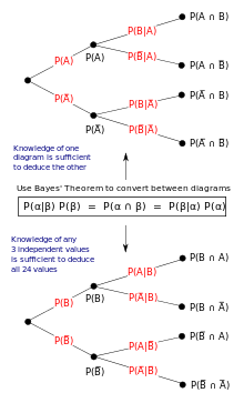
The role of Bayes' theorem is best visualized with tree diagrams, as shown to the right. The two diagrams partition the same outcomes by A and B in opposite orders, to obtain the inverse probabilities. Bayes' theorem serves as the link between these different partitionings.

Forms

Events

Simple form

For events A and B, provided that P(B) ≠ 0,

$P(A|B)={\frac {P(B|A)\,P(A)}{P(B)}}\cdot \,$

In many applications, for instance in Bayesian inference, the event B is fixed in the discussion, and we wish to consider the impact of its having been observed on our belief in various possible events A. In such a situation the denominator of the last expression, the probability of the given evidence B, is fixed; what we want to vary is A. Bayes theorem then shows that the posterior probabilities are proportional to the numerator:

$P(A|B)\propto P(A)\cdot P(B|A)\$ (proportionality over A for given B).

In words: posterior is proportional to prior times likelihood (see Lee, 2012, Chapter 1).

If events A₁, A₂, …, are mutually exclusive and exhaustive, i.e., one of them is certain to occur but no two can occur together, and we know their probabilities up to proportionality, then we can determine the proportionality constant by using the fact that their probabilities must add up to one. For instance, for a given event A, the event A itself and its complement ¬A are exclusive and exhaustive. Denoting the constant of proportionality by c we have

$P(A|B)=c\cdot P(A)\cdot P(B|A)\$ and $P(\neg A|B)=c\cdot P(\neg A)\cdot P(B|\neg A)\cdot$

Adding these two formulas we deduce that

$c={\frac {1}{P(A)\cdot P(B|A)+P(\neg A)\cdot P(B|\neg A)}}.$

Extended form

Often, for some partition {A_j} of the event space, the event space is given or conceptualized in terms of P(A_j) and P(B|A_j). It is then useful to compute P(B) using the law of total probability:

$P(B)={\sum _{j}P(B|A_{j})P(A_{j})},$

$\implies P(A_{i}|B)={\frac {P(B|A_{i})\,P(A_{i})}{\sum \limits _{j}P(B|A_{j})\,P(A_{j})}}\cdot$

In the special case where A is a binary variable:

$P(A|B)={\frac {P(B|A)\,P(A)}{P(B|A)P(A)+P(B|\neg A)P(\neg A)}}\cdot$

Random variables

Diagram illustrating the meaning of Bayes' theorem as applied to an event space generated by continuous random variables X and Y. Note that there exists an instance of Bayes' theorem for each point in the domain. In practice, these instances might be parametrized by writing the specified probability densities as a function of x and y.

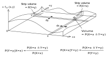
Consider a sample space Ω generated by two random variables X and Y. In principle, Bayes' theorem applies to the events A = {X = x} and B = {Y = y}. However, terms become 0 at points where either variable has finite probability density. To remain useful, Bayes' theorem may be formulated in terms of the relevant densities (see Derivation).

Simple form

If X is continuous and Y is discrete,

$f_{X}(x|Y=y)={\frac {P(Y=y|X=x)\,f_{X}(x)}{P(Y=y)}}.$

If X is discrete and Y is continuous,

$P(X=x|Y=y)={\frac {f_{Y}(y|X=x)\,P(X=x)}{f_{Y}(y)}}.$

If both X and Y are continuous,

$f_{X}(x|Y=y)={\frac {f_{Y}(y|X=x)\,f_{X}(x)}{f_{Y}(y)}}.$

Extended form

Diagram illustrating how an event space generated by continuous random variables X and Y is often conceptualized.

A continuous event space is often conceptualized in terms of the numerator terms. It is then useful to eliminate the denominator using the law of total probability. For f_Y(y), this becomes an integral:

$f_{Y}(y)=\int _{-\infty }^{\infty }f_{Y}(y|X=\xi )\,f_{X}(\xi )\,d\xi .$

Bayes' rule

Main article: Bayes' rule

Bayes' rule is Bayes' theorem in odds form.

$O(A_{1}:A_{2}|B)=O(A_{1}:A_{2})\cdot \Lambda (A_{1}:A_{2}|B)$

where

$\Lambda (A_{1}:A_{2}|B)={\frac {P(B|A_{1})}{P(B|A_{2})}}$

is called the Bayes factor or likelihood ratio

and the odds between two events is simply the ratio of the probabilities of the two events. Thus

$O(A_{1}:A_{2})={\frac {P(A_{1})}{P(A_{2})}}$,

$O(A_{1}:A_{2}|B)={\frac {P(A_{1}|B)}{P(A_{2}|B)}}$,

So the rule says that the posterior odds are the prior odds times the Bayes factor, or in other words, posterior is proportional to prior times likelihood.

Derivation

For events

Bayes' theorem may be derived from the definition of conditional probability:

$P(A|B)={\frac {P(A\cap B)}{P(B)}},{\text{ if }}P(B)\neq 0,\!$

$P(B|A)={\frac {P(A\cap B)}{P(A)}},{\text{ if }}P(A)\neq 0,\!$

$\implies P(A\cap B)=P(A|B)\,P(B)=P(B|A)\,P(A),\!$

$\implies P(A|B)={\frac {P(B|A)\,P(A)}{P(B)}},{\text{ if }}P(B)\neq 0.$

For random variables

For two continuous random variables X and Y, Bayes' theorem may be analogously derived from the definition of conditional density:

$f_{X}(x|Y=y)={\frac {f_{X,Y}(x,y)}{f_{Y}(y)}}$

$f_{Y}(y|X=x)={\frac {f_{X,Y}(x,y)}{f_{X}(x)}}$

$\implies f_{X}(x|Y=y)={\frac {f_{Y}(y|X=x)\,f_{X}(x)}{f_{Y}(y)}}.$

Examples

Frequentist example

Tree diagram illustrating frequentist example. R, C, P and P bar are the events representing rare, common, pattern and no pattern. Percentages in parentheses are calculated. Note that three independent values are given, so it is possible to calculate the inverse tree (see figure above).

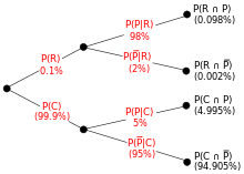
An entomologist spots what might be a rare subspecies of beetle, due to the pattern on its back. In the rare subspecies, 98% have the pattern, or P(Pattern|Rare) = 98%. In the common subspecies, 5% have the pattern. The rare subspecies accounts for only 0.1% of the population. How likely is the beetle having the pattern to be rare, or what is P(Rare|Pattern)?

From the extended form of Bayes' theorem (since any beetle can be only rare or common),

${\begin{aligned}P({\text{Rare}}|{\text{Pattern}})&={\frac {P({\text{Pattern}}|{\text{Rare}})P({\text{Rare}})}{P({\text{Pattern}}|{\text{Rare}})P({\text{Rare}})\,+\,P({\text{Pattern}}|{\text{Common}})P({\text{Common}})}}\\[8pt]&={\frac {0.98\times 0.001}{0.98\times 0.001+0.05\times 0.999}}\\[8pt]&\approx 1.9\%.\end{aligned}}$

Coin flip example

Concrete example from 5 August 2011 New York Times article by John Allen Paulos (quoted verbatim):

"Assume that you’re presented with three coins, two of them fair and the other a counterfeit that always lands heads. If you randomly pick one of the three coins, the probability that it’s the counterfeit is 1 in 3. This is the prior probability of the hypothesis that the coin is counterfeit. Now after picking the coin, you flip it three times and observe that it lands heads each time. Seeing this new evidence that your chosen coin has landed heads three times in a row, you want to know the revised posterior probability that it is the counterfeit. The answer to this question, found using Bayes’s theorem (calculation mercifully omitted), is 4 in 5. You thus revise your probability estimate of the coin’s being counterfeit upward from 1 in 3 to 4 in 5."

The calculation ("mercifully supplied") follows:

${\begin{aligned}P({\text{Biased coin}})&={\frac {1}{3}}\\[8pt]P({\text{Fair coin}})&={\frac {2}{3}}\\[8pt]P({\text{H}}|{\text{Fair coin}})&={\frac {1}{2}}\\[8pt]P({\text{HHH}}|{\text{Fair coin}})&={\frac {1}{8}}\\[8pt]P({\text{HHH}}|{\text{Biased coin}})&=1\\[8pt]P({\text{Biased coin}}|{\text{HHH}})&={\frac {P({\text{HHH}}|{\text{Biased coin}})P({\text{Biased coin}})}{P({\text{HHH}}|{\text{Biased coin}})P({\text{Biased coin}})+P({\text{HHH}}|{\text{Fair coin}})P({\text{Fair coin}})}}\\[8pt]&={\frac {1\times {\frac {1}{3}}}{1\times {\frac {1}{3}}+{\frac {1}{8}}\times {\frac {2}{3}}}}\quad =\quad {\frac {\frac {1}{3}}{\frac {10}{24}}}\quad =\quad {\frac {4}{5}}\\[8pt]\end{aligned}}$

Drug testing

Tree diagram illustrating drug testing example. U, U bar, "+" and "−" are the events representing user, non-user, positive result and negative result. Percentages in parentheses are calculated.

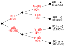
Suppose a drug test is 99% sensitive and 99% specific. That is, the test will produce 99% true positive results for drug users and 99% true negative results for non-drug users. Suppose that 0.5% of people are users of the drug. If a randomly selected individual tests positive, what is the probability he or she is a user?

${\begin{aligned}P({\text{User}}|{\text{+}})&={\frac {P({\text{+}}|{\text{User}})P({\text{User}})}{P({\text{+}}|{\text{User}})P({\text{User}})+P({\text{+}}|{\text{Non-user}})P({\text{Non-user}})}}\\[8pt]&={\frac {0.99\times 0.005}{0.99\times 0.005+0.01\times 0.995}}\\[8pt]&\approx 33.2\%\end{aligned}}$

Despite the apparent accuracy of the test, if an individual tests positive, it is more likely that they do not use the drug than that they do.

This surprising result arises because the number of non-users is very large compared to the number of users; thus the number of false positives (0.995%) outweighs the number of true positives (0.495%). To use concrete numbers, if 1000 individuals are tested, there are expected to be 995 non-users and 5 users. From the 995 non-users, 0.01 × 995 ≃ 10 false positives are expected. From the 5 users, 0.99 × 5 ≃ 5 true positives are expected. Out of 15 positive results, only 5, about 33%, are genuine.

Applications

Bayes Theorem is significantly important in inverse problem theory, where the a posteriori pdf is obtained from the product of prior pdf and the likelihood pdf. An important application is constructing computational models of oil reservoirs given the observed data.

Although Bayes theorem is commonly used to determine the probability of an event occurring, it can also be applied to verify someones credibility as a prognosticator. Many pundits claim to be able to predict the outcome of an event; political elections, trials, the weather and even sporting events. Larry Sabato, founder of Sabato’s Crystal Ball, is a perfect example. His website provides free political analysis and election predictions. His success at predictions has even led him to be called a “pundit with an opinion for every reporter’s phone call.” We even have Punxsutawney Phil, the famous groundhog, who tells us whether or not we can expect a longer winter or an early spring. Bayes theorem tells us the difference between who’s on a hot streak and who is what they claim to be.

Let’s say we live in an area where everyone gambles on the outcome of coin flips. Because of that, there is a big business for predicting coin flips. Suppose that 5% of predictors can actually win in the long run, and 80% of those are winners over a 2 year period. 95% of predictors are pretenders who are just guessing, and 20% of them are winners over a 2 year period (everyone gets lucky once in a while). This means that 82.6% of bettors who are winners over a 2 year period are actually long term losers who are winning above their real average.

History

Bayes' theorem was named after the Reverend Thomas Bayes (1701–61), who studied how to compute a distribution for the probability parameter of a binomial distribution (in modern terminology). His friend Richard Price edited and presented this work in 1763, after Bayes' death, as An Essay towards solving a Problem in the Doctrine of Chances. The French mathematician Pierre-Simon Laplace reproduced and extended Bayes' results in 1774, apparently quite unaware of Bayes' work. Stephen Stigler suggested in 1983 that Bayes' theorem was discovered by Nicholas Saunderson some time before Bayes. However, this interpretation has been disputed.

Further reading

• McGrayne, Sharon Bertsch (2011). The Theory That Would Not Die: How Bayes' Rule Cracked the Enigma Code, Hunted Down Russian Submarines & Emerged Triumphant from Two Centuries of Controversy. Yale University Press. ISBN 978-0-300-18822-6.
• Andrew Gelman, John B. Carlin, Hal S. Stern, and Donald B. Rubin (2003), "Bayesian Data Analysis", Second Edition, CRC Press.
• Charles M. Grinstead and J. Laurie Snell (1997), "Introduction to Probability (2nd edition)", American Mathematical Society (free pdf available [1].
• Pierre-Simon Laplace. (1774/1986), "Memoir on the Probability of the Causes of Events", Statistical Science 1(3):364–378.
• Peter M. Lee (2012), "Bayesian Statistics: An Introduction", Wiley.
• Rosenthal, Jeffrey S. (2005): "Struck by Lightning: the Curious World of Probabilities". Harper Collings.
• Stephen M. Stigler (1986), "Laplace's 1774 Memoir on Inverse Probability", Statistical Science 1(3):359–363.
• "Bayes formula", Encyclopedia of Mathematics, EMS Press, 2001 [1994]
• Stone, JV (2013). Chapter 1 of book "Bayes’ Rule: A Tutorial Introduction", University of Sheffield, Psychology.

External links

• The Theory That Would Not Die by Sharon Bertsch McGrayne New York Times Book Review by John Allen Paulos on 5 August 2011
• Visual explanation of Bayes using trees (video)
• Bayes' frequentist interpretation explained visually (video)
• Earliest Known Uses of Some of the Words of Mathematics (B). Contains origins of "Bayesian", "Bayes' Theorem", "Bayes Estimate/Risk/Solution", "Empirical Bayes", and "Bayes Factor".
• Weisstein, Eric W. "Bayes' Theorem". MathWorld.
• Bayes' theorem at PlanetMath.
• Bayes Theorem and the Folly of Prediction
• A tutorial on probability and Bayes’ theorem devised for Oxford University psychology students
• An Intuitive Explanation of Bayes' Theorem by Eliezer S. Yudkowsky