Evolutionary landscape

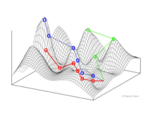
An evolutionary landscape is a metaphor; a construct used to think about and visualize the processes of evolution (e.g. natural selection and genetic drift) acting on a biological entity ( e.g., a gene, protein, population, species). This entity can be viewed as searching or moving through a search space. For example, the search space of a gene would be all possible nucleotide sequences. The search space is only part of an evolutionary landscape. The final component is the "y-axis," which is usually fitness. Each value along the search space can result in a high or low fitness for the entity. If small movements through search space causes small changes in fitness are relatively small, then the landscape is considered smooth. Smooth landscapes happen when most fixed mutations have little to no effect on fitness, which is what one would expect with the neutral theory of molecular evolution. In contrast, if small movements result in large changes in fitness, then the landscape is said to be rugged. In either case, movement tends to be toward areas of higher fitness, though usually not the global optima.

What exactly constitutes an "evolutionary landscape" is confused in the literature. The term evolutionary landscape is often used interchangeably with adaptive landscape and fitness landscape, though other authors distinguish between them. As discussed below, different authors have different definitions of adaptive and fitness landscapes. Additionally, there is large disagreement whether it should be used as a visual metaphor disconnected from the underlying math, a tool for evaluating models of evolution, or a model in and of itself used to generate hypotheses and predictions. Clearly, the field of biology, specifically evolutionary biology and population genetics, needs to come to a consensus of what an evolutionary landscape is and how it should be used.

History

Pre-Wright

According to McCoy (1979), the first evolutionary landscape was presented by Armand Janet of Toulon, France in 1895. In Janet's evolutionary landscape, a species is represented as a point or an area on a polydimensional surface of phenotypes, which is reduced to two dimensions for simplicity. The size of the population is proportional to the amount of variation within the population. Natural selection (the influence of the exterior features) is represented by a vector. Unlike the evolutionary landscapes of those who would follow, in Janet's concept, natural selection pulls species toward the minima instead of the maxima. This is because the y-axis doesn't represent fitness but stability. One important aspect of Janet's evolutionary landscape (versus Wright's) is that the landscape changes as the environment changes.

Wrightian Landscapes

Credit for the first evolutionary landscape typically goes to Sewall Wright, and his idea has arguably had a much larger audience and greater influence on the field of evolutionary biology. In his 1932 paper, Wright presents the concept of an evolutionary landscape composed of a polydimensional array of gene(allele) or genotype frequencies and an axis of fitness, which served as a visual metaphor to explain his shifting balance theory. Similarly to Janet, Wright felt the landscape could be reduced to two dimensions for simplicity. (This is one of the greatest criticisms, which are discussed below.) Populations are represented by areas, with the size of the area corresponding to the amount of genetic diversity within the population. Natural selection drives populations toward maxima, while drift represents wandering and could potentially cause a peak shift. Movement across the landscape represented changes in gene frequencies. This landscape was represented as a series of contour lines, much like a topological map; while selection kept or moved a biological entity to a peak, genetic drift allowed different peaks to be explored.

In 1944, Simpson expanded Wright's landscape to include phenotypes. Now, the landscape was a means of visualizing the "relationship between selection, structure, and adaptation." Unlike Wright, Simpson used the landscape to speak on both natural selection and genetic drift. Uphill movements are due to positive selection, and downhill movements are due to negative selection. The size and shape fo the peak indicated the relative specificity of selection, i.e. a sharp and high peak indicates highly specific selection. Another difference between Simpson's and Wright's landscapes is the level at which evolution is acting. For Wright, a population geneticist, only populations of a species were shown. In Simpson's figures, the circles drawn represent all of Equidae. The most important difference is that in Simposon's model, the landscape could vary through time while in Wright's model, the landscape was static. It is interesting to note that Wright reviewed Simpson's work (Tempo and Mode in Evolution) and did not object to Simpson's use of evolutionary landscapes. In later writings, Simpson referred to peaks as adaptive zones. In a series of papers Russell Lande developed a mathematical model for Simpson's phenotypic landscape. Lande reconciled Wright's population level view with Simpson's use of higher taxomonic levels. Lande considers fitness peaks to be determined by the environment and thus represent ecological niches or adaptive zones for a population. Clusters of peaks inhabited by phenotypically similar populations can be viewed as higher taxonomic levels.

Molecular Era

The concept of evolutionary landscapes changed once more as we entered the era of molecular evolution. It is claimed Maynard Smith (1970) is the first to visualize protein evolution as a network of proteins one mutational step away from others. However, for this to be true, there must be pathways between functional proteins. Acknowledging the work of Kimura, King, and Jukes (the neutral theory of molecular evolution), Maynard Smith realized the proteins along such pathways could have equal functionality or be neutral. In other words, not all moves in evolution are "uphill." In 1984, Gillespie adapted the concept of evolutionary landscapes to nucleotide sequences and so visualized the "mutational landscape" whereby all nucleotide sequences are one mutational step away from another, which is remarkably similar and yet fundamentally different from Wright's original concept. This conceptual shift, along with the development of vast computational power, has allowed evolutionary landscapes to move from being a simple visual metaphor to a working model of evolution. As one might expect, this has drawn heavy criticism and generated much research.

Hypothetical evolutionary landscape. The horizontal axes represent the biological parameters being measures (i.e. component of phenotype, genotype, nucleotide sequence combinations) and the vertical axis represents fitness. This particular example is a typical evolutionary landscape with peaks (lighter areas) and valleys (darker areas) generated from a shuffled dataset concerning the lichen Physcia millegrana.

Criticisms

One of the first criticisms (or at least difficulty) with evolutionary landscapes is their dimensionality. Wright recognized that true landscapes can have thousands of dimensions, but he also felt reducing those dimensions to two was acceptable since his point in doing so was to simply convey a complex idea. As a visual metaphor, this might be a valid reduction; however, the work of Gavrilets has shown that taking the high dimensionality of evolutionary landscapes into consideration may matter. In a high-dimensional framework, the peaks and valleys disappear and are replaced with hypervolume areas of high fitness and low fitness, which can be visualized as curved surfaces and holes in a 3-D landscape. While this does not affect visualization of the landscape per se (i.e. holes are equivalent to valleys), it does affect the underlying mathematical model and the predicted outcomes.

Hypothetical evolutionary landscape. The horizontal axes represent the biological parameters being measures (i.e. component of phenotype, genotype, nucleotide sequence combinations) and the vertical axis represents fitness. This particular landscape is an exaggerated example of Gavrilet's holey landscape.

The work of Gavrilets, along with other issues, has prompted Kaplan (2008) to propose abandoning the metaphor of evolutionary landscapes (which he calls adaptive or fitness landscapes). Kaplan (2008) has 6 main criticisms of the metaphor: (1) it has no explanatory power, (2) its lacks a relevant mathematical model, (3) it has no heuristic role, (4) it is imprecise, (5) it confuses more than it explains, (6) and there is no longer a reason to keep thinking in 2D or 3D when we have the computational power to consider higher dimensionality. Others feel Kaplan's criticisms are not warranted because he (and others) want evolutionary landscapes to meet the standards of a mathematical model; however, the landscape metaphor is just that, a metaphor. It has heuristic value as a metaphorical tool allowing one to visualize and evaluate the common core of assumptions in an evolutionary model. . While Kaplan (2008) wishes to discard the idea of landscapes all together, Massimo Pigliucci is less drastic. He acknowledges four categories of landscapes: fitness landscapes, adaptive landscapes, fitness surfaces, and morphospaces. Fitness landscapes are those similar to what Wright (1932) proposed (called an adaptive and fitness landscapes below). Adaptive landscapes are the phenotypic landscapes proposed by Simpson (1944), and fitness surfaces are the phenotypic landscapes with Lande's mathematical models applied to them. Morphospaces, pioneered by Raup (1966), are phenotypic landscapes developed a priori using mathematical models onto which observed measurements are mapped. They lack a fitness axis, and are used to show the occupied areas within the potential phenotypic space. Pigliucci suggests we abandon Wrightian fitness landscapes. Adaptive landscapes and fitness surfaces can be used with caution, i.e. with the understanding they are not phenotypic versions of Wright's original concept and that they are fraught with potentially misleading assumptions. Finally, Pigliucci calls for further research into morphospaces due to their heuristic value but also their ability to generate understandable and testable hypotheses.

Types of Evolutionary Landscapes

Adaptive Landscapes

Adaptive landscapes represent populations (of biological entities) as a single point, and the axes correspond to frequencies of alleles or genotypes and the mean population fitness.

Visualization of two dimensions of a NK fitness landscape. The arrows represent various mutational paths that the population could follow while evolving on the fitness landscape.

Fitness Landscapes

Fitness landscapes represent populations (of biological entities) as clusters of points with each point representing a unique genotype. The axes correspond to the loci of those genotypes and the resulting mean population fitness.

Phenotypic Landscape

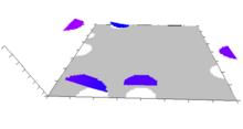
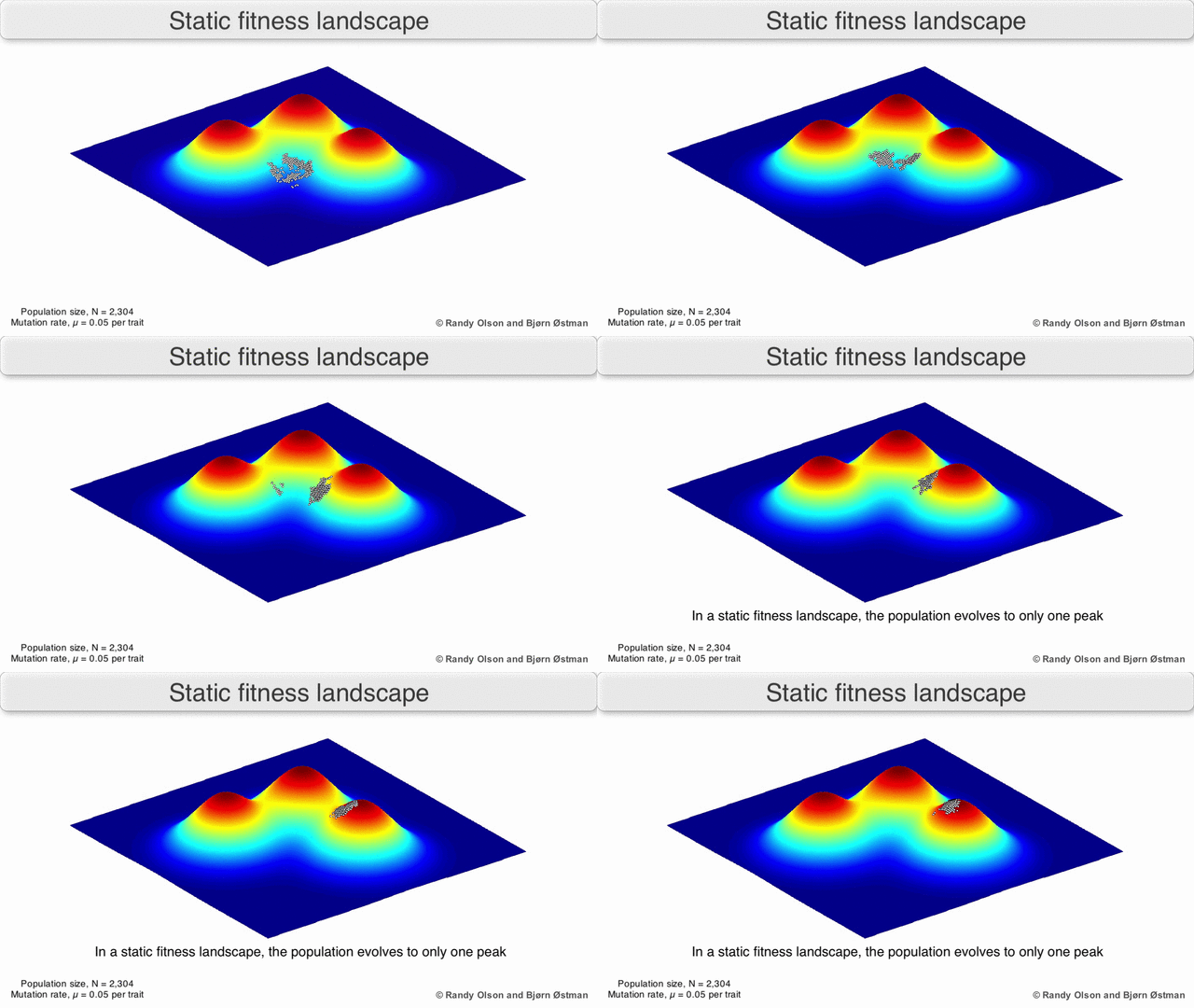
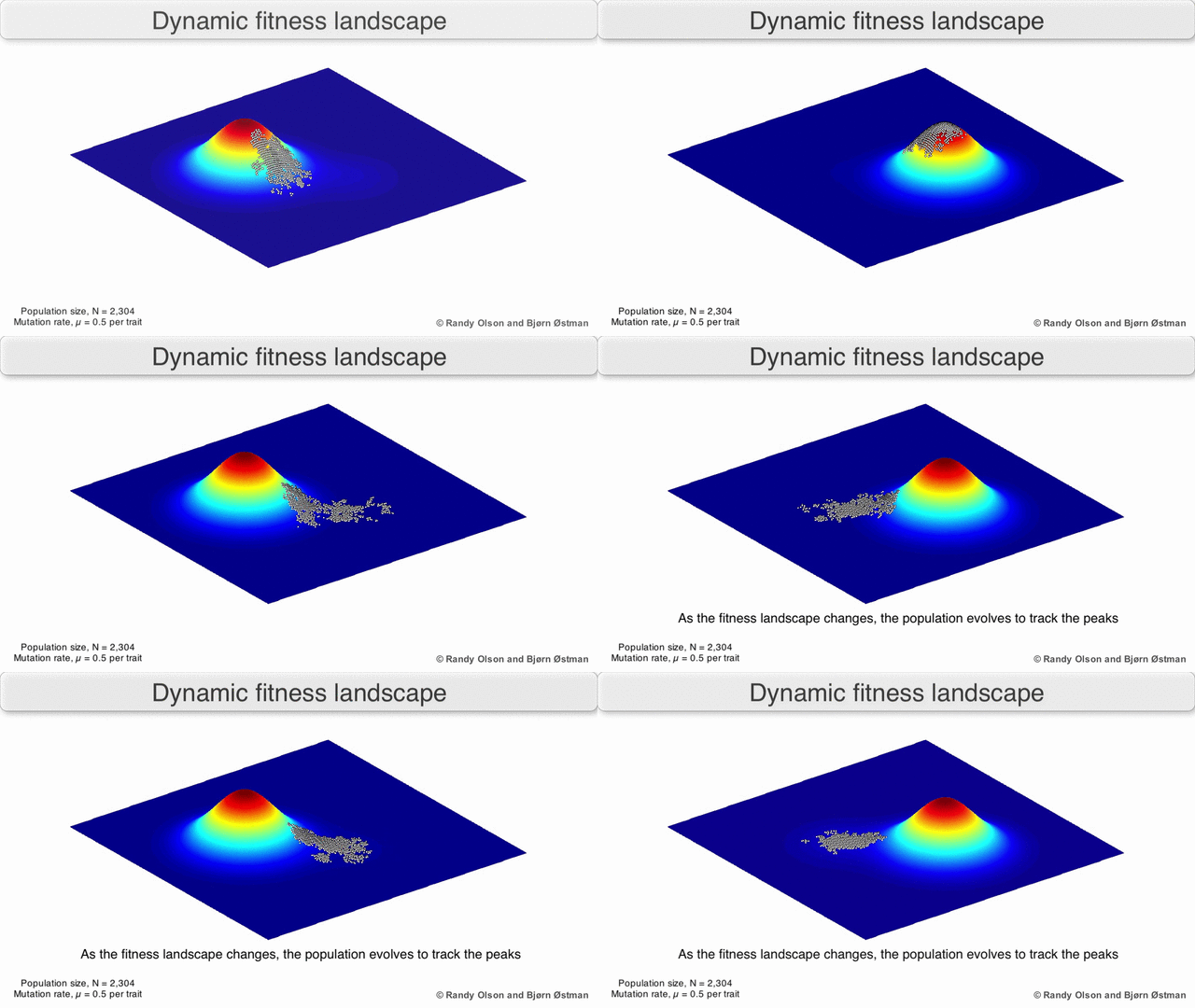
Phenotypic landscapes represent populations of species as clusters of points with each point representing a phenotype. The axes correspond to frequencies of phenotypes and the mean population fitness. See the visualizations below for examples of phenotypic landscapes.

Phenotypic Plasticity Landscape

Phenotypic plasticity landscapes depart from the other landscapes in that it does not use the mean population fitness. Instead, that axis represents characters (phenotypic traits) and other axes represent the underlying factors affecting the character.

Epigenetic Landscape

Epigenetic landscapes are "used to describe modal developmental tendency and major deviations" with a "space of abstract variables."

Morphospaces

Morphospaces also lack a dimension of fitness. Instead, their axes are mathematical models of phenotypic traits developed a priori to observational measurements. Observational measurements are then mapped onto the resulting surface to indicate areas of possible phenotypic space occupied by the species under consideration. .

Applications to Genomics

The increase of computational power and ease of sequencing has allowed for the concept of evolutionary landscapes to be taken from a purely conceptual metaphor to something that can be modeled and explored. This is especially true of the field of genomics. One good example is the research article "The Evolutionary Landscape of Cytosolic Microbial Sensors in Humans." In their study, Vasseur et al were interested in the evolution of the innate immune system; specifically, they wished to map the genetic diversity--the occupied evolutionary landscape--and patterns of selection and diversification--the movements made and being made along that landscape--of the nod-like receptor (NLRs) family of the pattern-recognition receptors (PRRs) that drive the innate immune response. These genes are responsible for detecting patterns/chemicals (e.g. chitin, oxidative stress) associated with invading microbes, tissue damage, and stress. To achieve this, they sequenced 21 genes from 185 humans and used several statistical methods to examine patterns of selection and diversification. The NLR family can be divided into two sub-families--the NALP subfamily and the NOD/IPAF sub-family. The authors found that the NALP family was under strong purifying selection and exhibited low genetic and functional diversity. They hypothesize this is because these genes have vital, non-redundant roles. Evidence in favor for this hypothesis comes from the independent discovery of rare alleles with mutations in two of the genes leading to a severe inflammatory disease and pregnancy complications. The NOD/IPAF family seems to have evolved under relaxed selection and exhibits a fair amount of genetic and functional diversity. The authors also found evidence of positive selection. The gene with the strongest positive selection was NLRP1, which has two haplotypes undergoing selective sweeps. The first haplotype is seven amino acids in strong linkage disequilibrium. This haplotype is global and seems to be moving toward fixation, which started in Asia and is still occurring in Europe and Africa. The second haplotype is restricted to Europe and is not in linkage disequilibrium with the global haplotype. This European haplotype carries with it a mutation associated with autoimmune diseases. The authors hypothesize another mutation in the haplotype is what selection is acting on and this deleterious mutation is simply hitchhiking along with it.

The second example comes from a paper titled "Synonymous Genes Explore Different Evolutionary Landscapes." (This article is publically available; see the citation below.) The authors of this paper are broadly interested in the ability of a protein to evolve. They specifically wanted to know how synonymous substitutions affected the evolutionary landscape of a protein. To do this, they used a program called the Evolutionary Landscape Printer to design a synonymous version of the antibiotic resistance gene aac(6')-IB. A synonymous protein has the same amino acid sequence but a different nucleotide sequences. Thus, a synonymous protein has the same function and fitness value but a different surrounding evolutionary landscape. Basically, this is a way to jump peaks without actually moving. The landscape of the original protein and the synonymous copy were explored computationally with Monte Carlo simulations and error-prone PCR. The PCR products were then inserted into competent E. coli cells and screened for novel antibiotic resistance. They found that the two proteins gave rise to very different novel phenotypes that, theoretically, are unreachable by the other. From their results, the authors concluded that synonymous codons allow for a wider exploration of the local evolutionary landscape, and that their method increases the odds of finding an advantageous mutation, which is useful for predicting how a population might change and for designing better organisms for industry.

External links

Examples of Visualized Evolutionary Landscapes

• Video: Using fitness landscapes to visualize evolution in action
• BEACON Blog--Evolution 101: Fitness Landscapes
• Pleiotrophy Blog--an interesting discussion of Sergey Gavrilets's contributions
• Pup Fish Evolution--UC Davis
• Evolution 101--Shifting Balance Theory (Figure at bottom of page)

Further Reading

• Counterbalance: Evolution as movement through a fitness landscape--an interesting (if flawed) discussion of evolution and fitness landscapes
• Example of the use of Evolutionary Landscapes in thinking & speaking about evolution

References

- ^ a b c d e f g Wright, Sewall (1932) The Roles of Mutation, Inbreeding, Crossbreeding, and Selection in Evolution. Proceedings of the Sixth International Congress of Genetics 1: 356-366
- ^ Wright, Sewall (1988) Surfaces of Selective Value Revisited. The American Naturalist 131(1):115-123
- ^ Lee, Carol E. & Gelebiuk, Gregory W. (2008) Evolutionary origins of invasive populations. "Evolutionary Applications" 1: 427-448.
- ^ a b McCoy J. Wynne. 1979. The Origin of the "Adaptive Landscape" Concept. The American Naturalist 113(4):610-613.
- ^ a b c d e f g h Dietrich MR & Skipper RA. 2012 "A Shifting Terrain: A Brief History of the Adaptive Landscape." In: The Adaptive Landscape in Evolutionary Biology. eds. Erik Svensson & Ryan Calsbeek Oxford Press.
- ^ a b c Simpson, GG. 1944. Tempo and Mode in Evolution Columbia University Press, New York.
- ^ a b c d Lande, R. (1976) Natural selection and random genetic drift in phenotypic evolution. Evolution 30: 314-334.
- ^ Lande, R. (1979) Effective Deme Sizes During Long-Term Evolution Estimated from Rates of Chromosomal Rearrangement. Evolution 33:234-251
- ^ The Adaptive Landscape in Evolutionary Biology. Eds. Erik Svensson & Ryan Calsbeek. 2012
- ^ a b c d e f g h Kaplan J. (2008) The end of the adaptive landscape metaphor? Bio Philos 23:625-638
- ^ Skipper RA & Dietrich MR. 2012 "Sewall Wright's adaptive landscape: Philosophical reflections on heuristic value." In: The Adaptive Landscape in Evolutionary Biology. eds. Erik Svensson & Ryan Calsbeek Oxford Press.
- ^ a b Pigliucci M 2012. "Landscapes, surfaces, and morphospaces: What are they good for?" In: The Adaptive Landscape in Evolutionary Biology. eds. Erik Svensson & Ryan Calsbeek Oxford Press.
- ^ a b Vasseur E, M Boniotto, E Patin, G Laval, H Quach, J Manry, B Crouau-Roy, & L Quintana-Murci. 2012. The Evolutionary Landscape of Cytosolic Microbial Sensors in Humans. The American Journal of Human Genetics 91:27-37.
- ^ a b c Cambray G & D Mazel. 2008. Synonymous Genes Explore Different Evolutionary Landscapes. PLoS Genetics 4(11).