
User:Tomasz.bartlomowicz/Conjoint R
conjoint: An Implementation of Conjoint Analysis Method | |
| Original author(s) | Andrzej Bąk and Tomasz Bartłomowicz |
|---|---|
| Initial release | October 2, 2011 |
| Stable release | 1.41
/ July 26, 2018 |
| Written in | R |
| Operating system | Windows, Linux/Unix, Mac OS |
| Platform | i386, x64 |
| Size | ~30 KB (binary version) |
| Available in | English |
| Type | Conjoint analysis, Statistical analysis |
| License | GNU GPL |
| Website | https://cran.r-project.org/package=conjoint |
conjoint R[1] – statistical software package for GNU R program. It contains the implementation of the traditional conjoint analysis method. It is written in R programming language as the development (module) of popular statistical software in the form of GNU R program, it also works with programs dedicated to R environment, such as: RStudio and Microsoft R Application Network.
The conjoint R package covers the set of functions[2] facilitating stated preference analysis based on empirical data representing consumers’ assessments of product or service profiles (the so-called total utilities, empirical utilities). Total utilities are subject to decomposition into the so-called part-worths utilities, which in further analysis are used to determine product or service importance, to define a product with optimal features, to separate segments of buyers with similar preferences, etc[3]. The decomposition is carried out based on the linear multiple regression model with dummy variables (lm function from stats R package [R Core Team 2018[4]]). The conjoint package allow as follows:
- estimation of conjoint analysis model parameters (part-worths utilities) in the cross-section of respondents (individual models) and the total sample (aggregated model),
- estimation of attributes’ importance (features describing profiles of products or services),
- estimation of the theoretical usefulness of complete product or service profiles,
- estimation of simulation profiles as market share,
- segmentation of respondents.
In addition, the package offers functions generating full and fractional (including orthogonal and effective) factorial design, necessary to prepare a proper questionnaire representing the tool for collecting data on respondents’ stated preferences using the conjoint analysis method.
The conjoint package source code is published based on GNU GPL licence rules. Binary versions are available for Windows, Macintosh systems and Unix systems (including Linux as the natural environment for GNU R project).
Requirements[edit]
The correct functioning of conjoint package requires installing GNU R basic version and also additional packages (e.g. AlgDesign R package [Wheeler 2015[5]] and others), which starting from 3.3.2 version of GNU R are automatically downloaded and installed including the conjoint package. The package can be downloaded and installed from the website of CRAN R repository (https://CRAN.R-project.org/package=conjoint[1]).
History and versions[edit]
The first version of conjoint package on CRAN server was available on October 2, 2011. Since then the package has been gradually developed and adapted to current standards, including various hardware platforms. The package can be installed on a computer with a 32-bit or a 64-bit processor. The package functionality is identical in both cases, with the exception of fractional factorial designs. In 32-bit systems it is possible to obtain a different fractional factorial design than in the case of 64-bit systems (it results from the numerical determinants of the machine word length and its impact on the seed of the random number generator, which is used in the procedure of fractional factorial design generation). The presented examples were developed using 64-bit processors working under the control of Windows 10 operating system.
Package functions[edit]
The current version of conjoint (1.41) package offers 16 functions, which allow for: model parameters estimation of conjoint analysis and respondents’ segmentation (functions: caModel, caSegmentation), estimation of theoretical part-worths utilities and total utilities in the cross-section of respondents (functions: caPartUtilities, caTotalUtilities), estimation of attributes’ importance and part-worths utilities of attributes’ levels at an aggregated level (functions: caImportance, caUtilities), and also – within the framework of simulation analysis – market share estimations of simulation profiles (functions: caBTL, caLogit, caMaxUtility). The special purpose functions include the function converting the empirical preference data set (caRankToScore function) and the functions which allow obtaining the aggregate results of the selected measurements and simulations (functions: Conjoint, ShowAllSimulations and ShowAllUtilities). In addition, the package offers tools supporting the design of a questionnaire survey, i.e. the construction of appropriate factorial designs, in particular to reduce the complete set of profiles in the form of fractional designs (orthogonal and effective). For this purpose the conjoint R package uses functions of AlgDesign R package [Wheeler 2015[5]]. The application of AlgDesign package functions in conjoint package is carried out in the form of functions, which allow generating orthogonal and effective fractional factorial designs and their encoding using artificial variables (functions: caFactorialDesign, caEncodedDesign andcaRecreatedDesign). In order to generate the appropriate factorial (full and fractional) design the data regarding the number of taken into account attributes (variables, features, factors) are sufficient and their levels (realizations, values, observations) as well as the names of attributes and levels. The detailed characteristics of all the available functions is provided in the official documentation [6] of conjoint R package and on other unofficial websites [7], [8], [9], [10] presenting the package application. The table presents the concise description of conjoint R package functions.
| Generating factorial designs and data conversion | |
|---|---|
| caFactorialDesign(data, type="null", cards=NA, seed=123) – the function determines the (full or fractional) factorial design with variable names and their levels | |
| caEncodedDesign(design) – the function encodes the factorial design obtained using caFactorialDesign function for the needs of conjoint module functioning | |
| caRecreatedDesign(attr.names, lev.numbers, z, prof.numbers) – the function recreates the fractional factorial design based on profile numbers from the full factorial design | |
| caRankToScore(y.rank) – the function transforms the empirical preference data measured on a rank scale into a data set in the form of point grades (on a positional scale) | |
| Estimation of individual part-worths utilities and theoretical total utilities (in the cross-section of respondents) | |
| caPartUtilities(y, x, z) – the function calculates the part-worths utility matrix of attribute levels in the cross-section of respondents (including an intercept) | |
| caTotalUtilities(y, x) – the function calculates the theoretical total utilities matrix of profiles in the cross-section of respondents | |
| Estimation of part-worths utilities of attributes’ levels (at an aggregated level) and the attributes’ importance level | |
| caUtilities(y, x, z) – the function calculates part-worths utilities of attributes’ levels at an aggregated level | |
| caImportance(y, x) – the function calculates an average relative “importance” of all attributes (as %) at an aggregated level | |
| Simulation analysis of market share | |
| caBTL(sym, y, x) – the function estimates market shares of simulation profiles based on the BTL probability model (Bradley-Terry-Luce Model) | |
| caLogit(sym, y, x) – the function estimates market shares of simulation profiles based on logit model | |
| caMaxUtility(sym, y, x) – the function estimates market shares of simulation profiles based on the maximum utility model | |
| Estimation of conjoint analysis model parameters and respondents’ segmentation | |
| caModel(y, x) – the function estimates conjoint analysis model parameters for an individual respondent | |
| caSegmentation(y, x, c=2) – the function performs respondents’ segmentation using k-means method | |
| Main results of conjoint analysis and simulation analysis | |
| Conjoint(y, x, z, y.type=”score”) – the function calculates basic results of conjoint analysis at an aggregated level | |
| ShowAllUtilities(y, x, z) – the function calculates all (part-worths and total) utilities available in the conjoint package | |
| ShowAllSimulations(sym, y, x) – the function estimates market shares of simulation profiles based on all simulation models available in the conjoint package | |
| Function arguments | |
| data | data describing the object of an experiment (product, service) – the set of attributes (factors) and their levels in the form of expand.grid function |
| type | optional parameter describing the type of generated factorial design (default type="null" – fractional design is generated with no specific criteria) |
| cards | optional parameter describing the number of generated profiles (default cards=NA – the number of profiles results from the type of generated factorial design) |
| seed | optional parameter describing the seed value of the random number generator (default seed=123) |
| design | factorial (fractional or full) experiment design |
| attr.names | vector representing names of attributes (factors) |
| lev.numbers | vector representing numbers of attributes’ (factors) levels |
| prof.numbers | vector representing numbers of reconstructed profiles |
| z | vector representing names of attributes’ (factors) levels |
| y.rank | matrix (or vector) of empirical preferences in the ranking form (the ranking data require transformation to rating data using caRankToScore function) |
| y | matrix (or vector) of empirical preferences (in the form of importance assessments on a rating or ranking scale) |
| x | matrix representing profiles (including names of attributes) |
| y.type | type of data about preferences – data in the form of profile importance assessments on a rating or ranking scale (default type is rating) |
| sym | matrix representing simulation profiles (including attributes’ names) |
| c | optional parameter specifying the number of segments (default c=2 – division into 2 segments) |
Package datasets[edit]
In version 1.41 of the conjoint R package there are 9 datasets that allow the presentation of using of the package functions. In each of datasets there are exemplary data describing: respondents' preferences (in the form of a data matrix or data vector), fractional factorial experiment design (in the form of a data matrix) and the names of individual variables' levels (in the form of data vector). In some datasets there is also design representing simulation profiles (in the form of a data matrix) that allows analysis of the market share of (products or services) profiles that were not included in the experiment design. Detailed characteristics of all datasets are available in the official documentation[6] of the conjoint package. The table presents a short description and the content of selected datasets of conjoint R package.
| Dataset name | Description | Content (with variables' names) |
|---|---|---|
| ice | Sample artificial data on a ranking scale (needs conversion) about preferences of ice-creams consumers. The product described by 4 attributes (with following attributes’ levels): flavour (chocolate, vanilla, strawberry), price ($1.50, $2.00, $2.50), container (cone, cup) and topping (yes, no). | ipref - matrix of preferences (6 respondents and 9 profiles), iprof - matrix of profiles (4 attributes and 9 profiles), ilevn - vector of names for the attributes' levels (10 levels). |
| tea | Sample data on a rating scale collected in 2007 about preferences of tea consumers. The product described by 4 attributes (with following attributes’ levels): price (low, medium, high), variety (black, green, red), kind (bags, granulated, leafy) and aroma (yes, no). | tprefm - matrix of preferences (100 respondents and 13 profiles), tpref - vector of preferences (length 1300), tprof - matrix of profiles (4 attributes and 13 profiles), tlevn - vector of names for the attributes' levels (11 levels), tsimp - matrix of simulation profiles (4 attributes and 4 profiles). |
| chocolate | Sample data on a rating scale collected in 2000 about preferences of chocolate consumers. The product described by 5 attributes (with following attributes’ levels): kind (milk, walnut, delicaties, dark), price (low, average, high), packing (paperback, hardback), weight (light, middle, heavy) and calorie (little, much). | cprefm - matrix of preferences (87 respondents and 16 profiles), cpref - vector of preferences (length 1392), cprof - matrix of profiles (5 attributes and 16 profiles), clevn - vector of names for the attributes' levels (14 levels), csimp - matrix of simulation profiles (5 attributes and 4 profiles). |
| journey | Sample data on a rating scale collected in 2015/2016 about preferences of tourists. The product described by 4 attributes (with following attributes’ levels): purpose (cognitive, vacation, health, business), form (organized, own), season (summer, winter) and accommodation (1-2-3 star hotel, 4-5 star hotel, guesthouse, hostel). | jpref - matrix of preferences (306 respondents and 14 profiles), jprof - matrix of profiles (4 attributes and 14 profiles), jlevn - vector of names for the attributes' levels (12 levels), csimp - matrix of simulation profiles (4 attributes and 5 profiles). |
> library(conjoint)
> data(tea)
> ls()
[1] "tlevn"  "tpref"  "tprefm" "tprof"  "tsimp"
> print(tprof)
   price variety kind aroma
1      3       1    1     1
2      1       2    1     1
3      2       2    2     1
4      2       1    3     1
5      3       3    3     1
6      2       1    1     2
7      3       2    1     2
8      2       3    1     2
9      3       1    2     2
10     1       3    2     2
11     1       1    3     2
12     2       2    3     2
13     3       2    3     2
> print(tsimp)
  price variety kind aroma
1     3       2    2     2
2     1       3    1     1
3     2       3    3     2
4     3       1    2     1
> print(tlevn)
       levels
1         low
2      medium
3        high
4       black
5       green
6         red
7        bags
8  granulated
9       leafy
10        yes
11         no
> tpref[1:78,]
 [1]  8  1  1  3  9  2  7  2  2  2  2  3  4  0 10  3  5  1  4  8  6  2  9  7  5  2  4 10  3  5  4  1  2  0  0  1
[37]  8  9  7  6  7  4  9  6  3  7  4  8  5  2 10  9  5  1  7  8  6 10  7 10  6  6  6 10  7 10  1  1  5  1  0  0
[73]  0  0  0  0  1  1
> head(tprefm)
  profil1 profil2 profil3 profil4 profil5 profil6 profil7 profil8 profil9 profil10 profil11 profil12 profil13
1       8       1       1       3       9       2       7       2       2        2        2        3        4
2       0      10       3       5       1       4       8       6       2        9        7        5        2
3       4      10       3       5       4       1       2       0       0        1        8        9        7
4       6       7       4       9       6       3       7       4       8        5        2       10        9
5       5       1       7       8       6      10       7      10       6        6        6       10        7
6      10       1       1       5       1       0       0       0       0        0        0        1        1
Practical applications of conjoint R package[edit]
Example 1. Consumer preference analysis of ice-creams based on the data collected on the rank scale[edit]
Research construction[edit]
Declaration of the research variables (including the relevant variable levels): flavour (chocolate, vanilla, strawberry), price ($1.50, $2.00, $2.50), container (cone, cup) and topping (yes, no):
> library(conjoint)
> experiment<-expand.grid(
+ flavor=c("chocolate","vanilla","strawberry"),
+ price=c("$1.50","$2.00","$2.50"),
+ container=c("cone","cup"),
+ topping=c("yes","no"))
Determining fractional, orthogonal factorial design with variable names and their levels for the needs of questionnaire construction:
> factdesign<-caFactorialDesign(data=experiment,type="orthogonal")
> print(factdesign)
       flavor price container topping
2     vanilla $1.50      cone     yes
6  strawberry $2.00      cone     yes
10  chocolate $1.50       cup     yes
13  chocolate $2.00       cup     yes
17    vanilla $2.50       cup     yes
18 strawberry $2.50       cup     yes
25  chocolate $2.50      cone      no
30 strawberry $1.50       cup      no
32    vanilla $2.00       cup      no
Encoding variable levels of the fractional design:
> prof=caEncodedDesign(design=factdesign)
> print(prof)
   flavor price container topping
2       2     1         1       1
6       3     2         1       1
10      1     1         2       1
13      1     2         2       1
17      2     3         2       1
18      3     3         2       1
25      1     3         1       2
30      3     1         2       2
32      2     2         2       2
Verification (using covariance and correlation matrix) of the fractional design quality:
> print(round(cov(prof),5))
          flavor price container topping
flavor      0.75  0.00      0.00    0.00
price       0.00  0.75      0.00    0.00
container   0.00  0.00      0.25    0.00
topping     0.00  0.00      0.00    0.25
> print(round(cor(prof),5))
          flavor price container topping
flavor         1     0         0       0
price          0     1         0       0
container      0     0         1       0
topping        0     0         0       1
> print(det(cor(prof)))
[1] 1
Data loading[edit]
Loading from external files: data on empirical preferences, research design, variable names and their levels
> pref=read.csv2("ice_preferences.csv", header=TRUE)
> profiles=read.csv2("ice_profiles.csv", header=TRUE)
> levelnames=read.csv2("ice_levels.csv", header=TRUE)
> print(pref)
  profile1 profile2 profile3 profile4 profile5 profile6 profile7 profile8 profile9
1        1        6        2        7        8        4        3        9        5
2        3        4        9        8        1        5        7        6        2
3        3        5        1        6        8        9        2        7        4
4        1        4        2        8        9        5        7        6        3
5        2        6        3        7        8        1        4        5        9
6        2        5        9        6        7        8        3        4        1
> print(profiles)
  flavour price container topping
1       2     1         1       1
2       3     2         1       1
3       1     1         2       1
4       1     2         2       1
5       2     3         2       1
6       3     3         2       1
7       1     3         1       2
8       3     1         2       2
9       2     2         2       2
> print(levelnames)
       levels
1   chocolate
2     vanilla
3  strawberry
4       $1.50
5       $2.00
6       $2.50
7        cone
8         cup
9         yes
10         no
Data files in comma-separated values (.csv format) to be downloaded: ice_preferences.csv, ice_profiles.csv, ice_levels.csv
Change of data format about preferences from rank ordering (so-called ranking) into importance assessments (so-called rating):
> preferences=caRankToScore(y.rank=pref)
> print(preferences)
  profile1 profile2 profile3 profile4 profile5 profile6 profile7 profile8 profile9
1        9        4        8        3        2        6        7        1        5
2        7        6        1        2        9        5        3        4        8
3        7        5        9        4        2        1        8        3        6
4        9        6        8        2        1        5        3        4        7
5        8        4        7        3        2        9        6        5        1
6        8        5        1        4        3        2        7        6        9
Measurement of preferences on an individual level (for selected respondents)[edit]
Conjoint analysis model estimation for the 1-st respondent:
> caModel(preferences[1,],profiles)

Call:
lm(formula = frml)

Residuals:
         1          2          3          4          5          6          7          8          9
 6.667e-01 -6.667e-01  1.500e+00 -1.500e+00 -2.833e+00  2.833e+00  2.591e-16 -2.167e+00  2.167e+00

Coefficients:
                     Estimate Std. Error t value Pr(>|t|)
(Intercept)            5.2500     1.4633   3.588   0.0697 .
factor(x$flavour)1     1.0000     1.8509   0.540   0.6431
factor(x$flavour)2     0.3333     1.8509   0.180   0.8737
factor(x$price)1       1.0000     1.8509   0.540   0.6431
factor(x$price)2      -1.0000     1.8509  -0.540   0.6431
factor(x$container)1   1.2500     1.3882   0.900   0.4629
factor(x$topping)1     0.5000     1.3882   0.360   0.7532
---
Signif. codes:  0 ‘***’ 0.001 ‘**’ 0.01 ‘*’ 0.05 ‘.’ 0.1 ‘ ’ 1

Residual standard error: 3.926 on 2 degrees of freedom
Multiple R-squared:  0.4861,    Adjusted R-squared:  -1.056
F-statistic: 0.3153 on 6 and 2 DF,  p-value: 0.8851
Determining relative importance of variables (attributes) for the 1-st respondent:
> importance=caImportance(y=preferences[1,],x=profiles)
> print(importance)
[1] 29.79 25.53 31.91 12.77
Measurement of preferences on an aggregated level (in the cross-section of respondents)[edit]
Measurement of part-worths utilities:
> partutilities=caPartUtilities(y=preferences,x=profiles,z=levelnames)
> print(partutilities)
     intercept chocolate vanilla strawberry  $1.50  $2.00  $2.50 cone   cup   yes    no
[1,]     5.250     1.000   0.333     -1.333  1.000 -1.000  0.000 1.25 -1.25  0.50 -0.50
[2,]     5.083    -3.000   3.000      0.000 -1.000  0.333  0.667 0.25 -0.25  0.00  0.00
[3,]     5.583     2.000   0.000     -2.000  1.333  0.000 -1.333 1.25 -1.25 -0.50  0.50
[4,]     5.167    -0.667   0.667      0.000  2.000  0.000 -2.000 0.75 -0.75  0.25 -0.25
[5,]     5.000     0.333  -1.333      1.000  1.667 -2.333  0.667 0.75 -0.75  0.75 -0.75
[6,]     6.000    -1.000   1.667     -0.667  0.000  1.000 -1.000 1.25 -1.25 -1.75  1.75
Measurement of total utilities:
> totalutilities=caTotalUtilities(y=preferences,x=profiles)
> print(totalutilities)
      [,1]  [,2]  [,3]  [,4]  [,5]  [,6] [,7]  [,8]   [,9]
[1,] 8.333 4.667 6.500 4.500 4.833 3.167    7 3.167  2.833
[2,] 7.333 5.667 0.833 2.167 8.500 5.500    3 3.833  8.167
[3,] 7.667 4.333 7.167 5.833 2.500 0.500    8 4.167  4.833
[4,] 8.833 6.167 6.000 4.000 3.333 2.667    3 6.167  4.833
[5,] 6.833 5.167 7.000 3.000 4.333 6.667    6 6.167 -0.167
[6,] 7.167 5.833 2.000 3.000 3.667 1.333    7 5.833  9.167
Summary of the most important preference measurement results using the Conjoint function:
> Conjoint(y=preferences,x=profiles,z=levelnames)

Call:
lm(formula = frml)

Residuals:
    Min      1Q  Median      3Q     Max
-3,9444 -1,6944  0,0833  1,3333  5,6944

Coefficients:
                     Estimate Std. Error t value Pr(>|t|)
(Intercept)            5,3472     0,3747  14,269   <2e-16 ***
factor(x$flavour)1    -0,2222     0,4740  -0,469   0,6414
factor(x$flavour)2     0,7222     0,4740   1,524   0,1343
factor(x$price)1       0,8333     0,4740   1,758   0,0853 .
factor(x$price)2      -0,3333     0,4740  -0,703   0,4854
factor(x$container)1   0,9167     0,3555   2,578   0,0131 *
factor(x$topping)1    -0,1250     0,3555  -0,352   0,7267
---
Signif. codes:  0 ‘***’ 0,001 ‘**’ 0,01 ‘*’ 0,05 ‘.’ 0,1 ‘ ’ 1

Residual standard error: 2,463 on 47 degrees of freedom
Multiple R-squared:  0,2079,    Adjusted R-squared:  0,1068
F-statistic: 2,057 on 6 and 47 DF,  p-value: 0,07656

[1] "Part worths (utilities) of levels (model parameters for whole sample):"
       levnms    utls
1   intercept  5,3472
2   chocolate -0,2222
3     vanilla  0,7222
4  strawberry    -0,5
5       $1.50  0,8333
6       $2.00 -0,3333
7       $2.50    -0,5
8        cone  0,9167
9         cup -0,9167
10        yes  -0,125
11         no   0,125
[1] "Average importance of factors (attributes):"
[1] 35,13 31,39 20,43 13,05
[1] Sum of average importance:  100
[1] "Chart of average factors importance"
-
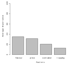 Fig. 2. The chart of variables (attributes) importance
 -
 Fig. 3. The chart of preference levels of flavour variable
 -
 Fig. 4. The chart of preference levels of price variable
 -
 Fig. 5. The chart of preference levels of container variable
 -
 Fig. 6. The chart of preference levels of topping variable


Example 2. Tourists’ preference measurement based on the data collected in the form of grades on an interval scale[edit]
Research construction[edit]
Declaration of the research variables (including the relevant variable levels): purpose (cognitive, vacation, health, business), form (organized, own), season (summer, winter), accommodation (1-2-3 star hotel, 4-5 star hotel, guesthouse, hostel):
> library(conjoint)
> journey<-expand.grid(purpose=c("cognitive","vacation","health","business"),
+ form=c("own","organized"),
+ season=c("summer","winter"),
+ accommodation=c("1-2-3 star hotel","4-5 star hotel","guesthouse","hostel"))
Determining fractional factorial design with variable names and their levels for the needs of questionnaire construction:
> journeyfactdesign<-caFactorialDesign(data=journey,type="fractional")
> journeyfactdesign
     purpose      form season    accommodation
1  cognitive       own summer 1-2-3 star hotel
8   business organized summer 1-2-3 star hotel
10  vacation       own winter 1-2-3 star hotel
15    health organized winter 1-2-3 star hotel
19    health       own summer   4-5 star hotel
21 cognitive organized summer   4-5 star hotel
30  vacation organized winter   4-5 star hotel
34  vacation       own summer       guesthouse
39    health organized summer       guesthouse
41 cognitive       own winter       guesthouse
48  business organized winter       guesthouse
54  vacation organized summer           hostel
60  business       own winter           hostel
61 cognitive organized winter           hostel
Encoding variable levels of the fractional design:
> prof=caEncodedDesign(design=journeyfactdesign)
> prof
   purpose form season accommodation
1        1    1      1             1
8        4    2      1             1
10       2    1      2             1
15       3    2      2             1
19       3    1      1             2
21       1    2      1             2
30       2    2      2             2
34       2    1      1             3
39       3    2      1             3
41       1    1      2             3
48       4    2      2             3
54       2    2      1             4
60       4    1      2             4
61       1    2      2             4
Data loading[edit]
Loading from external files: data on empirical preferences, research design, variable names, their levels and simulation profiles
> preferences=read.csv2("journey_preferences.csv", header=TRUE)
> profiles=read.csv2("journey_profiles.csv", header=TRUE)
> levelnames=read.csv2("journey_levels.csv", header=TRUE)
> simulations=read.csv2("journey_simulations.csv", header=TRUE)
> print(head(preferences))
  profile01 profile02 profile03 profile04 profile05 profile06 profile07 profile08 profile09 profile10 profile11 profile12 profile13 profile14
1         0        10         0        10        10         8         4         5        10         2         4         0         0         6
2        10         0        10         3         7         9         2         7         4         0         8        10         3         7
3         8         2         6         9         7         9         0         1         8         5         0         0         0         5
4         8        10         1         6         3         0         3         1         8         4         7         4         1        10
5         3         4         8        10        10         1        10         4         9         4        10         0         7        10
6         5         1         8         3        10         0         9         5         3        10        10         4         1         8
> print(profiles)
   purpose form season accommodation
1        1    1      1             1
2        4    2      1             1
3        2    1      2             1
4        3    2      2             1
5        3    1      1             2
6        1    2      1             2
7        2    2      2             2
8        2    1      1             3
9        3    2      1             3
10       1    1      2             3
11       4    2      2             3
12       2    2      1             4
13       4    1      2             4
14       1    2      2             4
> print(levelnames)
             levels
1         cognitive
2          vacation
3            health
4          business
5         organized
6               own
7            summer
8            winter
9  1-2-3 star_hotel
10   4-5 star_hotel
11       guesthouse
12           hostel
> print(simulations)
  purpose form season accommodation
1       2    2      1             1
2       2    1      1             2
3       3    2      2             2
4       1    1      1             4
5       4    1      2             3
Data files in comma-separated values (.csv format) to be downloaded: journey_preferences.csv, journey_profiles.csv, journej_levels.csv, journey_simulations.csv
Measurement of preferences (on an individual and aggregated level)[edit]
Measurement of part-worths utilities (in the cross-section of respondents):
> partutilities=caPartUtilities(y=preferences,x=profiles,z=levelnames)
> print(head(partutilities))
     intercept cognitive vacation health business organized    own summer winter 1-2-3 star_hotel 4-5 star_hotel guesthouse hostel
[1,]     4.938    -0.937   -2.687  3.639   -0.014    -1.562  1.562  0.692 -0.692            0.063          1.639      0.313 -2.014
[2,]     5.625     0.875    1.625 -0.827   -1.673     0.250 -0.250  1.058 -1.058            0.125         -0.452     -0.875  1.202
[3,]     4.187     2.563   -2.437  3.341   -3.466     0.063 -0.063  0.135 -0.135            2.062         -0.034     -0.688 -1.341
[4,]     4.375     1.125   -2.125  0.788    0.212    -1.625  1.625  0.346 -0.346            1.875         -2.962      0.625  0.462
[5,]     6.688    -2.187   -1.187  3.534   -0.159    -0.062  0.062 -2.385  2.385           -0.437          1.034      0.062 -0.659
[6,]     5.500     0.250    1.000  0.202   -1.452     0.750 -0.750 -1.808  1.808           -1.250          1.202      1.500 -1.452
Measurement of total utilities (in the cross-section of respondents):
> totalutilities=caTotalUtilities(y=preferences,x=profiles)
> print(head(totalutilities))
      [,1]  [,2]  [,3]   [,4]  [,5]  [,6]  [,7]  [,8]   [,9] [,10]  [,11] [,12]  [,13] [,14]
[1,] 3.192 7.240 0.058  9.510 9.346 7.894 4.760 1.692 11.144 2.058  6.106 2.490  0.654 2.856
[2,] 7.933 4.885 6.567  3.615 5.654 6.856 5.490 7.683  4.731 4.817  1.769 9.260  4.346 6.394
[3,] 9.010 2.856 3.740  9.394 7.692 6.788 1.519 1.260  6.913 5.990 -0.163 0.481 -0.692 5.212
[4,] 6.096 8.433 2.154  8.317 0.923 4.510 0.567 1.596  7.760 4.154  6.490 4.683  3.077 7.240
[5,] 1.615 3.769 7.385 12.231 8.808 3.212 8.981 3.115  7.962 6.885  9.038 2.519  8.192 6.288
[6,] 3.442 0.240 7.808  5.510 5.846 4.394 8.760 6.942  4.644 9.808  6.606 2.490  5.154 5.356
Determining the relative importance of features (for the respondent No.306):
> importance=caImportance(y=preferences[306,],x=profiles)
> print(importance)
[1] 41.97 18.11 13.37 26.56
Summary of the most important preference measurement results using the Conjoint function (for the respondent No. 306):
> Conjoint(preferences[306,],profiles,levelnames)

Call:
lm(formula = frml)

Residuals:
        1         2         3         4         5         6         7         8         9        10        11        12        13        14
 2,192308 -2,009615  2,557692 -2,740385  0,346154 -0,355769  0,009615 -3,307692  2,394231 -1,442308  2,355769  0,740385 -0,346154 -0,394231

Coefficients:
                         Estimate Std. Error t value Pr(>|t|)
(Intercept)                4,9375     0,8685   5,685  0,00235 **
factor(x$purpose)1         1,3125     1,4003   0,937  0,39165
factor(x$purpose)2        -0,4375     1,4003  -0,312  0,76733
factor(x$purpose)3         1,7356     1,6158   1,074  0,33184
factor(x$form)1            0,9375     0,8685   1,080  0,32966
factor(x$season)1         -0,6923     0,8617  -0,803  0,45823
factor(x$accommodation)1   1,3125     1,4003   0,937  0,39165
factor(x$accommodation)2   0,7356     1,6158   0,455  0,66802
factor(x$accommodation)3  -1,4375     1,4003  -1,027  0,35171
---
Signif. codes:  0 ‘***’ 0,001 ‘**’ 0,01 ‘*’ 0,05 ‘.’ 0,1 ‘ ’ 1

Residual standard error: 3,107 on 5 degrees of freedom
Multiple R-squared:  0,6034,    Adjusted R-squared:  -0,0311
F-statistic: 0,951 on 8 and 5 DF,  p-value: 0,549

[1] "Part worths (utilities) of levels (model parameters for whole sample):"
             levnms    utls
1         intercept  4,9375
2         cognitive  1,3125
3          vacation -0,4375
4            health  1,7356
5          business -2,6106
6         organized  0,9375
7               own -0,9375
8            summer -0,6923
9            winter  0,6923
10 1-2-3 star_hotel  1,3125
11   4-5 star_hotel  0,7356
12       guesthouse -1,4375
13           hostel -0,6106
[1] "Average importance of factors (attributes):"
[1] 41,97 18,11 13,37 26,56
[1] Sum of average importance:  100,01
[1] "Chart of average factors importance"
Summary of the most important preference measurement results using the Conjoint function (in the cross-section of respondents):
> Conjoint(y=preferences,x=profiles,z=levelnames)

Call:
lm(formula = frml)

Residuals:
    Min      1Q  Median      3Q     Max
-5,4460 -3,0144 -0,0949  2,7758  5,9051

Coefficients:
                          Estimate Std. Error t value Pr(>|t|)
(Intercept)               4,979371   0,052578  94,704  < 2e-16 ***
factor(x$purpose)1        0,139093   0,084780   1,641   0,1009
factor(x$purpose)2        0,146446   0,084780   1,727   0,0842 .
factor(x$purpose)3        0,437924   0,097823   4,477 7,78e-06 ***
factor(x$form)1          -0,070057   0,052578  -1,332   0,1828
factor(x$season)1        -0,094834   0,052172  -1,818   0,0692 .
factor(x$accommodation)1 -0,136234   0,084780  -1,607   0,1081
factor(x$accommodation)2 -0,028171   0,097823  -0,288   0,7734
factor(x$accommodation)3  0,005923   0,084780   0,070   0,9443
---
Signif. codes:  0 ‘***’ 0,001 ‘**’ 0,01 ‘*’ 0,05 ‘.’ 0,1 ‘ ’ 1

Residual standard error: 3,291 on 4275 degrees of freedom
Multiple R-squared:  0,01474,   Adjusted R-squared:  0,0129
F-statistic: 7,994 on 8 and 4275 DF,  p-value: 9,444e-11

[1] "Part worths (utilities) of levels (model parameters for whole sample):"
             levnms    utls
1         intercept  4,9794
2         cognitive  0,1391
3          vacation  0,1464
4            health  0,4379
5          business -0,7235
6         organized -0,0701
7               own  0,0701
8            summer -0,0948
9            winter  0,0948
10 1-2-3 star_hotel -0,1362
11   4-5 star_hotel -0,0282
12       guesthouse  0,0059
13           hostel  0,1585
[1] "Average importance of factors (attributes):"
[1] 38,62 13,30 13,97 34,11
[1] Sum of average importance:  100
[1] "Chart of average factors importance"
-
 Fig. 7. The chart of variables (attributes) importance
 -
 Fig. 8. The chart of preference levels of purpose variable
 -
 Fig. 9. The chart of preference levels of form variable
 -
 Fig. 10. The chart of preference levels of season variable
 -
 Fig. 11. The chart of preference levels of accommodation variable


Segmentation of respondents[edit]
Segmentation using k-means method - the default division into 2 segments:
> segments<-caSegmentation(preferences,profiles)
> print(segments$seg)
K-means clustering with 2 clusters of sizes 149, 157

Cluster means:
      [,1]     [,2]     [,3]    [,4]     [,5]     [,6]     [,7]     [,8]     [,9]    [,10]    [,11]    [,12]    [,13]    [,14]
1 6.025658 3.686060 5.200852 5.08743 4.808973 5.088503 4.263604 4.948477 4.835148 6.630383 4.290691 3.291765 3.721228 4.973577
2 3.670554 4.482898 4.837408 5.78621 5.618357 5.043720 6.210573 4.984248 5.933051 3.743459 4.555803 7.127006 5.120497 5.886217

Clustering vector:
  [1] 2 2 1 1 2 1 1 1 2 1 2 1 2 1 1 2 1 1 1 2 1 1 2 1 2 2 1 2 1 2 1 2 1 1 1 1 2 1 1 1 1 1 2 2 2 1 1 2 2 1 2 1 1 1 1 1 1 2 2 1 2 1 1 2 2 1 1 2 2 1 1 2 1
 [74] 1 2 1 1 2 2 2 2 2 2 2 2 2 2 2 2 1 2 2 2 2 1 2 1 2 2 2 2 1 1 2 2 2 2 1 2 2 2 2 2 1 1 2 2 1 2 2 1 1 1 2 2 1 1 2 1 1 2 1 1 2 2 2 1 1 1 2 1 2 2 1 2 2
[147] 2 2 2 2 2 2 1 2 2 1 1 1 2 1 2 2 2 1 2 2 2 2 1 2 1 2 1 2 2 1 2 1 2 2 2 2 2 1 2 2 2 2 2 2 2 2 1 1 2 1 1 1 2 1 1 2 1 2 2 1 2 2 2 2 2 1 1 1 2 1 1 2 1
[220] 1 2 2 2 2 2 2 1 2 1 1 2 1 1 1 2 2 2 1 1 1 2 1 1 1 2 2 1 1 1 1 2 2 2 1 1 2 2 1 2 1 2 1 2 1 1 2 1 1 1 1 1 2 2 1 1 1 2 2 2 1 2 1 1 1 1 2 1 1 1 2 1 1
[293] 2 1 1 1 1 2 2 1 1 2 1 1 1 1

Within cluster sum of squares by cluster:
[1] 12885.85 11758.15
 (between_SS / total_SS =  10.6%)

Available components:

[1] "cluster"      "centers"      "totss"        "withinss"     "tot.withinss" "betweenss"    "size"         "iter"         "ifault"
Segmentation using k-means method – division into 3 segments:
> segments<-caSegmentation(preferences,profiles,c=3)
> print(segments$seg)
K-means clustering with 3 clusters of sizes 104, 97, 105

Cluster means:
      [,1]     [,2]     [,3]     [,4]     [,5]     [,6]     [,7]     [,8]     [,9]    [,10]    [,11]    [,12]    [,13]    [,14]
1 5.263000 3.860952 4.155269 7.124625 7.068404 4.630298 3.522462 3.895212 6.864673 5.561519 4.159365 3.494365 4.614288 5.160567
2 5.602402 3.695979 6.044505 3.409691 3.393330 5.303907 5.746031 6.161680 3.526845 6.583165 4.676763 4.284897 3.513887 4.706402
3 3.650619 4.695133 4.913667 5.664390 5.089067 5.276390 6.539390 4.924429 5.675200 3.416048 4.460514 7.908229 5.120457 6.399800

Clustering vector:
  [1] 1 3 1 1 1 2 2 2 2 1 3 1 1 2 2 3 1 1 2 1 1 2 1 2 3 3 2 2 1 3 2 3 2 2 2 2 3 2 1 2 2 1 2 3 3 2 2 3 3 1 3 2 2 1 2 2 1 3 1 2 3 1 2 3 2 1 1 3 1 2 2 1 2
 [74] 2 1 1 1 1 3 3 3 3 3 3 3 1 3 2 2 1 3 3 3 3 1 3 2 3 3 3 3 2 2 3 3 2 3 1 3 3 3 1 2 2 2 3 3 2 3 3 2 1 2 3 3 2 2 1 1 1 3 1 1 3 1 1 2 3 2 3 2 3 3 1 3 1
[147] 1 1 3 3 1 3 2 2 1 2 1 2 3 1 3 3 1 2 1 3 3 3 1 3 2 3 1 3 3 1 3 2 2 1 3 1 3 2 3 3 3 3 2 3 3 3 2 1 3 2 2 2 1 1 1 3 1 3 3 1 2 3 3 1 2 1 1 2 3 2 2 3 1
[220] 2 3 3 3 3 3 2 2 2 2 1 2 2 2 1 1 1 3 2 1 1 3 1 1 2 3 3 1 2 1 1 1 1 1 1 2 3 1 1 3 2 2 1 1 1 1 1 2 2 1 2 1 3 3 1 1 1 3 1 3 2 3 2 1 2 1 3 2 1 1 1 2 2
[293] 3 2 1 2 2 3 3 2 1 3 1 2 1 1

Within cluster sum of squares by cluster:
[1] 8321.434 7030.496 7021.380
 (between_SS / total_SS =  18.9%)

Available components:

[1] "cluster"      "centers"      "totss"        "withinss"     "tot.withinss" "betweenss"    "size"         "iter"         "ifault"
Visualization of the division into 3 segments:
> summary(segments)
     Length Class  Mode
segm    9   kmeans list
util 4284   -none- numeric
sclu  306   -none- numeric

> require(fpc)
> plotcluster(segments$util,segments$sclu)

> require(fpc)
> require(broom)
> require(ggplot2)
> dcf<-discrcoord(segments$util,segments$sclu)
> assignments<-augment(segments$segm,dcf$proj[,1:2])
> ggplot(assignments)+geom_point(aes(x=X1,y=X2,color= .cluster))+labs(color="Cluster Assignment",title="K-Means Clustering Results")
-
![Fig. 9. Division into 3 segments (using plotcluster function of fpc R package [Hennig 2018[11]])](//upload.wikimedia.org/wikipedia/commons/thumb/7/74/Trip_ce2_3clusters.svg/220px-Trip_ce2_3clusters.svg.png) Fig. 9. Division into 3 segments (using plotcluster function of fpc R package [Hennig 2018[11]])
Fig. 9. Division into 3 segments (using plotcluster function of fpc R package [Hennig 2018[11]]) -
![Fig. 10. Division into 3 segments (using ggplot function of ggplot2 R package [Wickham et al. 2018[12]])](//upload.wikimedia.org/wikipedia/commons/thumb/d/d7/Trip_ce3_3clusters.svg/220px-Trip_ce3_3clusters.svg.png) Fig. 10. Division into 3 segments (using ggplot function of ggplot2 R package [Wickham et al. 2018[12]])
Fig. 10. Division into 3 segments (using ggplot function of ggplot2 R package [Wickham et al. 2018[12]])
![Fig. 9. Division into 3 segments (using plotcluster function of fpc R package [Hennig 2018[11]])](/wiki/File:Trip_ce2_3clusters.svg)
![Fig. 10. Division into 3 segments (using ggplot function of ggplot2 R package [Wickham et al. 2018[12]])](/wiki/File:Trip_ce3_3clusters.svg)
[edit]
Market share analysis of simulation profiles using maximum utility model, BTL probability model (Bradley-Terry-Luce Model) and logit model:
> ShowAllSimulations(sym=simulations,y=preferences,x=profiles)
  TotalUtility MaxUtility BTLmodel LogitModel
1         4,96      20,26    19,31      17,51
2         4,93      11,44    20,01      15,72
3         5,55      31,05    22,32      29,02
4         5,11      24,84    20,77      23,07
5         4,29      12,42    17,59      14,68
References[edit]
- ^ a b Andrzej Bąk; Tomasz Bartłomowicz (2018-07-26). "conjoint: An Implementation of Conjoint Analysis Method". Retrieved 2018-07-26.
- ^ Andrzej Bąk; Tomasz Bartłomowicz (2012). "Conjoint analysis method and its implementation in conjoint R package". In Józef Pociecha; Reinhold Decker (eds.). Data analysis methods and its applications (PDF). Warszawa: C.H.Beck. pp. 239–248. ISBN 978-83-255-3458-5.
- ^ Eugeniusz Gatnar; Marek Walesiak (2009). Statystyczna analiza danych z wykorzystaniem programu R. Warszawa: Wydawnictwo Naukowe PWN. ISBN 978-83-01-15661-9.
- ^ R Core Team and contributors worldwide (2018-07-08). "stats: The R Stats Package". Retrieved 2018-07-07.
{{cite web}}:|author=has generic name (help) - ^ a b Bob Wheeler (2014-10-15). "AlgDesign: Algorithmic Experimental Design". Retrieved 2018-06-30.
- ^ a b Andrzej Bąk, Tomasz Bartłomowicz (2018-07-26). "Package 'conjoint' – manual" (PDF). Retrieved 2018-07-26.
- ^ Jinsuh Lee (2016-11-05). "Conjoint Analysis on R". Retrieved 2018-07-07.
- ^ Markus Burkhardt (2018-01-28). "R-Stutorials – 24 Conjoint-Analyse". Retrieved 2018-07-07.
- ^ Martin Müller (2018-04-01). "Market Research Using Conjoint Analysis In R". Retrieved 2018-07-07.
- ^ Holly Jones (2015). "Conjoint Analysis & Segmentation". Retrieved 2018-07-07.
- ^ Christian Hennig (2018-01-13). "fpc: Flexible Procedures for Clustering". Retrieved 2018-07-07.
- ^ Cite error: The named reference
ggplot2was invoked but never defined (see the help page).
External links[edit]
- Official website of conjoint R package (English)
- Documentation of conjoint R package on CRAN (English)
- Conjoint R package on YouTube (English)
- Conjoint R package on YouTube (German)
See also[edit]
Category:Mathematical software Category:Free statistical software Category:R (programming language) Category:GNU