Riemann sum

Four of the Riemann summation methods for approximating the area under curves. Right and left methods make the approximation using the right and left endpoints of each subinterval, respectively. Maximum and minimum methods make the approximation using the largest and smallest endpoint values of each subinterval, respectively. The values of the sums converge as the subintervals halve from top-left to bottom-right.

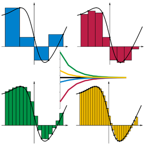
In mathematics, a Riemann sum is a certain kind of approximation of an integral by a finite sum. It is named after nineteenth century German mathematician Bernhard Riemann. One very common application is approximating the area of functions or lines on a graph, but also the length of curves and other approximations.

The sum is calculated by partitioning the region into shapes (rectangles, trapezoids, parabolas, or cubics) that together form a region that is similar to the region being measured, then calculating the area for each of these shapes, and finally adding all of these small areas together. This approach can be used to find a numerical approximation for a definite integral even if the fundamental theorem of calculus does not make it easy to find a closed-form solution.

Because the region filled by the small shapes is usually not exactly the same shape as the region being measured, the Riemann sum will differ from the area being measured. This error can be reduced by dividing up the region more finely, using smaller and smaller shapes. As the shapes get smaller and smaller, the sum approaches the Riemann integral.

Definition

Let $f:[a,b]\rightarrow \mathbb {R}$ be a function defined on a closed interval $[a,b]$ of the real numbers, $\mathbb {R}$, and

$P=\left\{[x_{0},x_{1}],[x_{1},x_{2}],\dots ,[x_{n-1},x_{n}]\right\}$⁠,

be a partition of I, where

$a=x_{0}<x_{1}<x_{2}<\cdots <x_{n}=b$.

A Riemann sum $S$ of f over I with partition P is defined as

$S=\sum _{i=1}^{n}f(x_{i}^{*})\,\Delta x_{i}$

where $\Delta x_{i}=x_{i}-x_{i-1}$ and an $x_{i}^{*}\in [x_{i-1},x_{i}]$. Notice the use of "a" instead of "the" in the previous sentence. Another way of thinking about this asterisk is that you are choosing some random point in this slice, and it does not matter which one; as the difference or width of the slices approaches zero, the difference between any two points in our rectangle slice approaches zero as well. This is due to the fact that the choice of $x_{i}^{*}$ in the interval $[x_{i-1},x_{i}]$ is arbitrary, so for any given function f defined on an interval I and a fixed partition P, one might produce different Riemann sums depending on which $x_{i}^{*}$ is chosen, as long as $x_{i-1}\leq x_{i}^{*}\leq x_{i}$ holds true.

Some specific types of Riemann sums

Specific choices of $x_{i}^{*}$ give us different types of Riemann sums:

• If $x_{i}^{*}=x_{i-1}$ for all i, then S is called a left rule or left Riemann sum.
• If $x_{i}^{*}=x_{i}$ for all i, then S is called a right rule or right Riemann sum.
• If $x_{i}^{*}=(x_{i}+x_{i-1})/2$ for all i, then S is called the midpoint rule or middle Riemann sum.
• If $f(x_{i}^{*})=\sup f([x_{i-1},x_{i}])$ (that is, the supremum of f over $[x_{i-1},x_{i}]$), then S is defined to be an upper Riemann sum or upper Darboux sum.
• If $f(x_{i}^{*})=\inf f([x_{i-1},x_{i}])$ (that is, the infimum of f over $[x_{i-1},x_{i}]$), then S is defined to be an lower Riemann sum or lower Darboux sum.

All these methods are among the most basic ways to accomplish numerical integration. Loosely speaking, a function is Riemann integrable if all Riemann sums converge as the partition "gets finer and finer".

While not technically a Riemann sum, the average of the left and right Riemann sums is the trapezoidal sum and is one of the simplest of a very general way of approximating integrals using weighted averages. This is followed in complexity by Simpson's rule and Newton–Cotes formulas.

Any Riemann sum on a given partition (that is, for any choice of $x_{i}^{*}$ between $x_{i-1}$ and $x_{i}$) is contained between the lower and upper Darboux sums. This forms the basis of the Darboux integral, which is ultimately equivalent to the Riemann integral.

Methods

The four methods of Riemann summation are usually best approached with partitions of equal size. The interval [a, b] is therefore divided into n subintervals, each of length

$\Delta x={\frac {b-a}{n}}.$

The points in the partition will then be

$a,a+\Delta x,a+2\,\Delta x,\ldots ,a+(n-2)\,\Delta x,a+(n-1)\,\Delta x,b.$

Left Riemann sum

Left Riemann sum of x³ over [0,2] using 4 subdivisions

For the left Riemann sum, approximating the function by its value at the left-end point gives multiple rectangles with base Δx and height f(a + iΔx). Doing this for i = 0, 1, ..., n − 1, and adding up the resulting areas gives

$\Delta x\left[f(a)+f(a+\Delta x)+f(a+2\,\Delta x)+\cdots +f(b-\Delta x)\right].$

The left Riemann sum amounts to an overestimation if f is monotonically decreasing on this interval, and an underestimation if it is monotonically increasing.

Right Riemann sum

Right Riemann sum of x³ over [0,2] using 4 subdivisions

f is here approximated by the value at the right endpoint. This gives multiple rectangles with base Δx and height f(a + i Δx). Doing this for i = 1, ..., n, and adding up the resulting areas produces

$\Delta x\left[f(a+\Delta x)+f(a+2\,\Delta x)+\cdots +f(b)\right].$

The right Riemann sum amounts to an underestimation if f is monotonically decreasing, and an overestimation if it is monotonically increasing. The error of this formula will be

$\left\vert \int _{a}^{b}f(x)\,dx-A_{\mathrm {right} }\right\vert \leq {\frac {M_{1}(b-a)^{2}}{2n}}$,

where $M_{1}$ is the maximum value of the absolute value of $f^{\prime }(x)$ on the interval.

Midpoint rule

Midpoint Riemann sum of x³ over [0,2] using 4 subdivisions

Approximating f at the midpoint of intervals gives f(a + Δx/2) for the first interval, for the next one f(a + 3Δx/2), and so on until f(b − Δx/2). Summing up the areas gives

$\Delta x\left[f(a+{\tfrac {\Delta x}{2}})+f(a+{\tfrac {3\,\Delta x}{2}})+\cdots +f(b-{\tfrac {\Delta x}{2}})\right]$.

The error of this formula will be

$\left\vert \int _{a}^{b}f(x)\,dx-A_{\mathrm {mid} }\right\vert \leq {\frac {M_{2}(b-a)^{3}}{24n^{2}}}$,

where $M_{2}$ is the maximum value of the absolute value of $f^{\prime \prime }(x)$ on the interval.

Trapezoidal rule

Trapezoidal Riemann sum of x³ over [0,2] using 4 subdivisions

Main article: Trapezoidal rule

In this case, the values of the function f on an interval are approximated by the average of the values at the left and right endpoints. In the same manner as above, a simple calculation using the area formula

$A={\tfrac {1}{2}}h(b_{1}+b_{2})$

for a trapezium with parallel sides b₁, b₂ and height h produces

${\tfrac {1}{2}}\,\Delta x\left[f(a)+2f(a+\Delta x)+2f(a+2\,\Delta x)+2f(a+3\,\Delta x)+\cdots +f(b)\right].$

The error of this formula will be

$\left\vert \int _{a}^{b}f(x)\,dx-A_{\mathrm {trap} }\right\vert \leq {\frac {M_{2}(b-a)^{3}}{12n^{2}}},$

where $M_{2}$ is the maximum value of the absolute value of $f^{\prime \prime }(x)$.

The approximation obtained with the trapezoid rule for a function is the same as the average of the left hand and right hand sums of that function.

Connection with integration

For a one-dimensional Riemann sum over domain $[a,b]$, as the maximum size of a partition element shrinks to zero (that is the limit of the norm of the partition goes to zero), some functions will have all Riemann sums converge to the same value. This limiting value, if it exists, is defined as the definite Riemann integral of the function over the domain,

$\int _{a}^{b}\!f(x)\,dx=\lim _{\|\Delta x\|\rightarrow 0}\sum _{i=1}^{n}f(x_{i}^{*})\,\Delta x_{i}.$

For a finite-sized domain, if the maximum size of a partition element shrinks to zero, this implies the number of partition elements goes to infinity. For finite partitions, Riemann sums are always approximations to the limiting value and this approximation gets better as the partition gets finer. The following animations help demonstrate how increasing the number of partitions (while lowering the maximum partition element size) better approximates the "area" under the curve:

• 
  Left sum
• 
  Right sum
• 
  Middle sum

Since the red function here is assumed to be a smooth function, all three Riemann sums will converge to the same value as the number of partitions goes to infinity.

Example

Comparison of right hand sums of the function y = x² from 0 to 2 with the integral of it from 0 to 2.

A visual representation of the area under the curve y = x² for the interval from 0 to 2. Using antiderivatives this area is exactly 8/3.

Approximating the area under $y=x^{2}$ from 0 to 2 using right-rule sums. Notice that because the function is monotonically increasing, right-hand sums will always overestimate the area contributed by each term in the sum (and do so maximally).

The value of the Riemann sum under the curve y = x² from 0 to 2. As the number of rectangles increases, it approaches the exact area of 8/3.

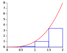
Taking an example, the area under the curve of y = x² between 0 and 2 can be procedurally computed using Riemann's method.

The interval [0, 2] is firstly divided into n subintervals, each of which is given a width of ${\tfrac {2}{n}}$; these are the widths of the Riemann rectangles (hereafter "boxes"). Because the right Riemann sum is to be used, the sequence of x coordinates for the boxes will be $x_{1},x_{2},\ldots ,x_{n}$. Therefore, the sequence of the heights of the boxes will be $x_{1}^{2},x_{2}^{2},\ldots ,x_{n}^{2}$. It is an important fact that $x_{i}={\tfrac {2i}{n}}$, and $x_{n}=2$.

The area of each box will be ${\tfrac {2}{n}}\times x_{i}^{2}$ and therefore the nth right Riemann sum will be:

${\begin{aligned}S&={\frac {2}{n}}\times \left({\frac {2}{n}}\right)^{2}+\cdots +{\frac {2}{n}}\times \left({\frac {2i}{n}}\right)^{2}+\cdots +{\frac {2}{n}}\times \left({\frac {2n}{n}}\right)^{2}\\&={\frac {8}{n^{3}}}\left(1+\cdots +i^{2}+\cdots +n^{2}\right)\\&={\frac {8}{n^{3}}}\left({\frac {n(n+1)(2n+1)}{6}}\right)\\&={\frac {8}{n^{3}}}\left({\frac {2n^{3}+3n^{2}+n}{6}}\right)\\&={\frac {8}{3}}+{\frac {4}{n}}+{\frac {4}{3n^{2}}}\end{aligned}}$

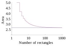
If the limit is viewed as n → ∞, it can be concluded that the approximation approaches the actual value of the area under the curve as the number of boxes increases. Hence:

$\lim _{n\to \infty }S=\lim _{n\to \infty }\left({\frac {8}{3}}+{\frac {4}{n}}+{\frac {4}{3n^{2}}}\right)={\frac {8}{3}}$

This method agrees with the definite integral as calculated in more mechanical ways:

$\int _{0}^{2}x^{2}\,dx={\frac {8}{3}}$

Because the function is continuous and monotonically increasing on the interval, a right Riemann sum overestimates the integral by the largest amount (while a left Riemann sum would underestimate the integral by the largest amount). This fact, which is intuitively clear from the diagrams, shows how the nature of the function determines how accurate the integral is estimated. While simple, right and left Riemann sums are often less accurate than more advanced techniques of estimating an integral such as the Trapezoidal rule or Simpson's rule.

The example function has an easy-to-find anti-derivative so estimating the integral by Riemann sums is mostly an academic exercise; however it must be remembered that not all functions have anti-derivatives so estimating their integrals by summation is practically important.

Higher dimensions

The basic idea behind a Riemann sum is to "break-up" the domain via a partition into pieces, multiply the "size" of each piece by some value the function takes on that piece, and sum all these products. This can be generalized to allow Riemann sums for functions over domains of more than one dimension.

While intuitively, the process of partitioning the domain is easy to grasp, the technical details of how the domain may be partitioned get much more complicated than the one dimensional case and involves aspects of the geometrical shape of the domain.

Two dimensions

In two dimensions, the domain, $A$ may be divided into a number of cells, $A_{i}$ such that $A=\cup _{i}A_{i}$. In two dimensions, each cell then can be interpreted as having an "area" denoted by $\Delta A_{i}$. The Riemann sum is

$S=\sum _{i=1}^{n}f(x_{i}^{*},y_{i}^{*})\,\Delta A_{i},$

where $(x_{i}^{*},y_{i}^{*})\in A_{i}$.

Three dimensions

In three dimensions, it is customary to use the letter $V$ for the domain, such that $V=\cup _{i}V_{i}$ under the partition and $\Delta V_{i}$ is the "volume" of the cell indexed by $i$. The three-dimensional Riemann sum may then be written as

$S=\sum _{i=1}^{n}f(x_{i}^{*},y_{i}^{*},z_{i}^{*})\,\Delta V_{i}$

with $(x_{i}^{*},y_{i}^{*},z_{i}^{*})\in V_{i}$.

Arbitrary number of dimensions

Higher dimensional Riemann sums follow a similar as from one to two to three dimensions. For an arbitrary dimension, n, a Riemann sum can be written as

$S=\sum _{i}f(P_{i}^{*})\,\Delta V_{i}$

where $P_{i}^{*}\in V_{i}$, that is, it's a point in the n-dimensional cell $V_{i}$ with n-dimensional volume $\Delta V_{i}$.

Generalization

In high generality, Riemann sums can be written

$S=\sum _{i}f(P_{i}^{*})\mu (V_{i})$

where $P_{i}^{*}$ stands for any arbitrary point contained in the partition element $V_{i}$ and $\mu$ is a measure on the underlying set. Roughly speaking, a measure is a function that gives a "size" of a set, in this case the size of the set $V_{i}$; in one dimension, this can often be interpreted as the length of the interval, in two dimensions, an area, in three dimensions, a volume, and so on.

See also

• Antiderivative
• Euler method and midpoint method, related methods for solving differential equations
• Lebesgue integral
• Riemann integral, limit of Riemann sums as the partition becomes infinitely fine
• Simpson's rule, a powerful numerical method more powerful than basic Riemann sums or even the Trapezoidal rule
• Trapezoidal rule, numerical method based on the average of the left and right Riemann sum

External links

• Weisstein, Eric W. "Riemann Sum". MathWorld.
• A simulation showing the convergence of Riemann sums

References

- ^ Hughes-Hallett, Deborah; McCullum, William G. (2005). Calculus (4th ed.). Wiley. p. 252.
{{cite book}}: Unknown parameter|displayauthors=ignored (|display-authors=suggested) (help) (Among many equivalent variations on the definition, this reference closely resembles the one given here.) - ^ a b c Hughes-Hallett, Deborah; McCullum, William G. (2005). Calculus (4th ed.). Wiley. p. 340.
So far, we have three ways of estimating an integral using a Riemann sum: 1. The left rule uses the left endpoint of each subinterval. 2. The right rule uses the right endpoint of each subinterval. 3. The midpoint rule uses the midpoint of each subinterval.
{{cite book}}: Unknown parameter|displayauthors=ignored (|display-authors=suggested) (help) - ^ a b c Ostebee, Arnold; Zorn, Paul (2002). Calculus from Graphical, Numerical, and Symbolic Points of View (Second ed.). p. M-33.
Left-rule, right-rule, and midpoint-rule approximating sums all fit this definition.
- ^ Swokowski, Earl W. (1979). Calculus with Analytic Geometry (Second ed.). Boston, MA: Prindle, Weber & Schmidt. pp. 821–822. ISBN 0-87150-268-2.
- ^ Ostebee, Arnold; Zorn, Paul (2002). Calculus from Graphical, Numerical, and Symbolic Points of View (Second ed.). p. M-34.
We chop the plane region R into m smaller regions R1, R2, R3, ..., Rm, perhaps of different sizes and shapes. The 'size' of a subregion Ri is now taken to be its area, denoted by ΔAi.
- ^ Swokowski, Earl W. (1979). Calculus with Analytic Geometry (Second ed.). Boston, MA: Prindle, Weber & Schmidt. pp. 857–858. ISBN 0-87150-268-2.
![{\displaystyle f:[a,b]\rightarrow \mathbb {R} }](https://wikimedia.org/api/rest_v1/media/math/render/svg/fc0d2d0b70573525d149ab82948308455d1853d0)
![{\displaystyle [a,b]}](https://wikimedia.org/api/rest_v1/media/math/render/svg/9c4b788fc5c637e26ee98b45f89a5c08c85f7935)
![{\displaystyle P=\left\{[x_{0},x_{1}],[x_{1},x_{2}],\dots ,[x_{n-1},x_{n}]\right\}}](https://wikimedia.org/api/rest_v1/media/math/render/svg/096b0a34cf6fae9227f91ca153b55cb9f60e4492)
![{\displaystyle x_{i}^{*}\in [x_{i-1},x_{i}]}](https://wikimedia.org/api/rest_v1/media/math/render/svg/dafeab86f1179399f11208ee27a15c76434aed3d)
![{\displaystyle [x_{i-1},x_{i}]}](https://wikimedia.org/api/rest_v1/media/math/render/svg/09cb12a889d47020c8ce7046a2eb60785e00c0b6)
![{\displaystyle f(x_{i}^{*})=\sup f([x_{i-1},x_{i}])}](https://wikimedia.org/api/rest_v1/media/math/render/svg/dff7dfd2109629595f3fdf32681f3e6f7009c047)
![{\displaystyle f(x_{i}^{*})=\inf f([x_{i-1},x_{i}])}](https://wikimedia.org/api/rest_v1/media/math/render/svg/a7b2f108cd78e38003810fff4cdccbdd4d37c77a)
![{\displaystyle \Delta x\left[f(a)+f(a+\Delta x)+f(a+2\,\Delta x)+\cdots +f(b-\Delta x)\right].}](https://wikimedia.org/api/rest_v1/media/math/render/svg/d39698586a053c8cb0750eb693c4f4f824634fc9)
![{\displaystyle \Delta x\left[f(a+\Delta x)+f(a+2\,\Delta x)+\cdots +f(b)\right].}](https://wikimedia.org/api/rest_v1/media/math/render/svg/b62a3d74a79890847931dae31aec437b8fe38fbf)
![{\displaystyle \Delta x\left[f(a+{\tfrac {\Delta x}{2}})+f(a+{\tfrac {3\,\Delta x}{2}})+\cdots +f(b-{\tfrac {\Delta x}{2}})\right]}](https://wikimedia.org/api/rest_v1/media/math/render/svg/8d3f332318381b31a3e68e5e8900e7f4964c0a9e)
![{\displaystyle {\tfrac {1}{2}}\,\Delta x\left[f(a)+2f(a+\Delta x)+2f(a+2\,\Delta x)+2f(a+3\,\Delta x)+\cdots +f(b)\right].}](https://wikimedia.org/api/rest_v1/media/math/render/svg/50854a88e6c67f444995d39a8455cefaf2e64dbd)