Lambert W function

The graph of W(x) for W > −4 and z < 6. The upper branch with W ≥ −1 is the function W₀ (principal branch), the lower branch with W ≤ −1 is the function W₋₁.

In mathematics, the Lambert W function, also called the omega function or product logarithm, is a set of functions, namely the branches of the inverse relation of the function z = f(W) = We^W where e^W is the exponential function and W is any complex number. In other words, the defining equation for W(z) is

$z=W(z)e^{W(z)}$

for any complex number z.

Since the function ƒ$\scriptstyle (\cdot )$ is not injective, the relation W is multivalued (except at 0). If we restrict attention to real-valued W, the complex variable z is then replaced by the real variable x, and the relation is defined only for x ≥ −1/e, and is double-valued on (−1/e, 0). The additional constraint W ≥ −1 defines a single-valued function W₀(x). We have W₀(0) = 0 and W₀(−1/e) = −1. Meanwhile, the lower branch has W ≤ −1 and is denoted W₋₁(x). It decreases from W₋₁(−1/e) = −1 to W₋₁(0⁻) = −∞.

The Lambert W relation cannot be expressed in terms of elementary functions. It is useful in combinatorics, for instance in the enumeration of trees. It can be used to solve various equations involving exponentials (e.g. the maxima of the Planck, Bose–Einstein, and Fermi–Dirac distributions) and also occurs in the solution of delay differential equations, such as y'(t) = a y(t − 1).

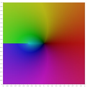
Main branch of the Lambert W function in the complex plane. Note the branch cut along the negative real axis, ending at −1/e. In this picture, the hue of a point z is determined by the argument of W(z) and the brightness by the absolute value of W(z).

Terminology

The two main branches $W_{0}$ and $W_{-1}$

The Lambert W-function is named after Johann Heinrich Lambert. The main branch W₀ is denoted by Wp in the Digital Library of Mathematical Functions and the branch W₋₁ is denoted by Wm there.

The notation convention chosen here (with W₀ and W₋₁) follows the canonical reference on the Lambert-W function by Corless, Gonnet, Hare, Jeffrey and Knuth.

History

Lambert first considered the related Lambert's Transcendental Equation in 1758, which led to a paper by Leonhard Euler in 1783 that discussed the special case of we^w. However the inverse of we^w was first described by Pólya and Szegő in 1925. The Lambert W function was "re-discovered" every decade or so in specialized applications but its full importance was not realized until the 1990s. When it was reported that the Lambert W function provides an exact solution to the quantum-mechanical double-well Dirac delta function model for equal charges—a fundamental problem in physics—Corless and developers of the Maple Computer algebra system made a library search to find that this function was in fact ubiquitous to nature.

Calculus

Derivative

By implicit differentiation, one can show that all branches of W satisfy the differential equation

$z(1+W){\frac {{\rm {d}}W}{{\rm {d}}z}}=W\quad {\text{for }}z\neq -1/e.$

(W is not differentiable for z = −1/e.) As a consequence, we get the following formula for the derivative of W:

${\frac {{\rm {d}}W}{{\rm {d}}z}}={\frac {W(z)}{z(1+W(z))}}\quad {\text{for }}z\not \in \{0,-1/e\}.$

Furthermore we have

$\left.{\frac {{\rm {d}}W}{{\rm {d}}z}}\right|_{z=0}=1.$

Antiderivative

The function W(x), and many expressions involving W(x), can be integrated using the substitution w = W(x), i.e. x = w e^w:

$\int W(x)\,{\rm {d}}x=x\left(W(x)-1+{\frac {1}{W(x)}}\right)+C.$

One consequence of which (using the fact that $W(e)=1$) is the identity:

$\int _{0}^{e}W(x)\,{\rm {d}}x=e-1$

Asymptotic expansions

The Taylor series of $W_{0}$ around 0 can be found using the Lagrange inversion theorem and is given by

$W_{0}(x)=\sum _{n=1}^{\infty }{\frac {(-n)^{n-1}}{n!}}\ x^{n}=x-x^{2}+{\frac {3}{2}}x^{3}-{\frac {8}{3}}x^{4}+{\frac {125}{24}}x^{5}-\cdots$

The radius of convergence is 1/e, as may be seen by the ratio test. The function defined by this series can be extended to a holomorphic function defined on all complex numbers with a branch cut along the interval (−∞, −1/e]; this holomorphic function defines the principal branch of the Lambert W function.

For large values of x, W₀ is asymptotic to

$W_{0}(x)=L_{1}-L_{2}+{\frac {L_{2}}{L_{1}}}+{\frac {L_{2}(-2+L_{2})}{2L_{1}^{2}}}+{\frac {L_{2}(6-9L_{2}+2L_{2}^{2})}{6L_{1}^{3}}}+{\frac {L_{2}(-12+36L_{2}-22L_{2}^{2}+3L_{2}^{3})}{12L_{1}^{4}}}+\cdots$

$W_{0}(x)=L_{1}-L_{2}+\sum _{\ell =0}^{\infty }\sum _{m=1}^{\infty }{\frac {(-1)^{\ell }\left[{\begin{matrix}\ell +m\\\ell +1\end{matrix}}\right]}{m!}}L_{1}^{-\ell -m}L_{2}^{m}$

where $L_{1}=\ln x$, $L_{2}=\ln \ln x$ and $\left[{\begin{matrix}\ell +m\\\ell +1\end{matrix}}\right]$ is a non-negative Stirling number of the first kind. Keeping only the first two terms of the expansion,

$W_{0}(x)=\ln x-\ln \ln x+o(1).$

The other real branch, $W_{-1}$, defined in the interval (−∞, −1/e], has an approximation of the same form as x approaches zero, with in this case $L_{1}=\ln(-x)$ and $L_{2}=\ln(-\ln(-x))$.

Integer and complex powers

Integer powers of $W_{0}$ also admit simple Taylor (or Laurent) series expansions at $0$

$W_{0}(x)^{2}=\sum _{n=2}^{\infty }{\frac {-2(-n)^{n-3}}{(n-2)!}}\ x^{n}=x^{2}-2x^{3}+4x^{4}-{\frac {25}{3}}x^{5}+18x^{6}-\cdots$

More generally, for $r\in \mathbb {Z} ,$, the Lagrange inversion formula gives

$W_{0}(x)^{r}=\sum _{n=r}^{\infty }{\frac {-r(-n)^{n-r-1}}{(n-r)!}}\ x^{n},$

which is, in general, a Laurent series of order r. Equivalently, the latter can be written in the form of a Taylor expansion of powers of $W_{0}(x)/x$

$\left({\frac {W_{0}(x)}{x}}\right)^{r}=\exp(-rW_{0}(x))=\sum _{n=0}^{\infty }{\frac {r(n+r)^{n-1}}{n!}}\ (-x)^{n},$

which holds for any $r\in \mathbb {C}$ and $|x|<e^{-1}$.

Special values

For any non-zero algebraic number x, W(x) is a transcendental number. We can show this by contradiction: If W(x) were non-zero and algebraic (note that if x is non-zero then W(x) must be non-zero as well), then by the Lindemann–Weierstrass theorem, e^W(x) must be transcendental, implying that x=W(x)e^W(x) must also be transcendental, contradicting the condition that x is algebraic.

$W\left(-{\frac {\pi }{2}}\right)={\frac {\pi }{2}}{\rm {i}}$

$W\left(-{\frac {\ln a}{a}}\right)=-\ln a\quad \left({\frac {1}{e}}\leq a\leq e\right)$

$W\left(-{\frac {1}{e}}\right)=-1$

$W\left(0\right)=0\,$

$W\left(1\right)=\Omega ={\frac {1}{\displaystyle \int _{-\infty }^{+\infty }{\frac {\,dt}{(e^{t}-t)^{2}+\pi ^{2}}}}}-1\approx 0.56714329\dots \,$ (the Omega constant)

$W\left(e\right)=1\,$

$W\left(-1\right)\approx -0.31813-1.33723{\rm {i}}\,$

$W'\left(0\right)=1\,$

Other formulas

There are several useful integration formulae involving the W function. Some of these include the following:

$\int _{0}^{\pi }W{\bigl (}2\cot ^{2}(x){\bigr )}\sec ^{2}(x)\;\mathrm {d} x=4{\sqrt {\pi }}$

$\int _{0}^{\infty }{\frac {W(x)}{x{\sqrt {x}}}}\mathrm {d} x=2{\sqrt {2\pi }}$

$\int _{0}^{\infty }W\left({\frac {1}{x^{2}}}\right)\;\mathrm {d} x={\sqrt {2\pi }}$

The second identity can be derived by making the substitution

$u=W(x)$

which gives

$x=ue^{u}$

${\frac {dx}{du}}=(u+1)e^{u}$

Thus

$\int _{0}^{\infty }{\frac {W(x)}{x{\sqrt {x}}}}\mathrm {d} x=\int _{0}^{\infty }{\frac {u}{ue^{u}{\sqrt {ue^{u}}}}}(u+1)e^{u}\mathrm {d} u$

$=\int _{0}^{\infty }{\frac {u+1}{\sqrt {ue^{u}}}}\mathrm {d} u$

$=\int _{0}^{\infty }{\frac {u+1}{\sqrt {u}}}{\frac {1}{\sqrt {e^{u}}}}\mathrm {d} u$

$=\int _{0}^{\infty }u^{\frac {1}{2}}e^{-{\frac {u}{2}}}\mathrm {d} u+\int _{0}^{\infty }u^{-{\frac {1}{2}}}e^{-{\frac {u}{2}}}\mathrm {d} u$

$=2\int _{0}^{\infty }(2w)^{\frac {1}{2}}e^{-w}\mathrm {d} w+2\int _{0}^{\infty }(2w)^{-{\frac {1}{2}}}e^{-w}\mathrm {d} w$ (by making the substitution $u=2w$)

$=2{\sqrt {2}}\int _{0}^{\infty }w^{\frac {1}{2}}e^{-w}\mathrm {d} w+{\sqrt {2}}\int _{0}^{\infty }w^{-{\frac {1}{2}}}e^{-w}\mathrm {d} w$

$=2{\sqrt {2}}\Gamma ({\frac {3}{2}})+{\sqrt {2}}\Gamma ({\frac {1}{2}})$

$=2{\sqrt {2}}({\frac {1}{2}}{\sqrt {\pi }})+{\sqrt {2}}({\sqrt {\pi }})$

$=2{\sqrt {2\pi }}$

The third identity may be derived from the second by making the substitution $u={\frac {1}{x^{2}}}$

Applications

Many equations involving exponentials can be solved using the W function. The general strategy is to move all instances of the unknown to one side of the equation and make it look like Y = Xe^X at which point the W function provides the value of the variable in X.

In other words :

$Y=Xe^{X}\;\Longleftrightarrow \;X=W(Y)$

Examples

Example 1

${\begin{aligned}2^{t}&=5t\\1&={\frac {5t}{2^{t}}}\\1&=5t\,e^{-t\ln 2}\\{\frac {1}{5}}&=t\,e^{-t\ln 2}\\{\frac {-\,\ln 2}{5}}&=(-\,t\,\ln 2)\,e^{(-t\ln 2)}\\W\left({\frac {-\ln 2}{5}}\right)&=-t\ln 2\\t&=-{\frac {W\left({\frac {-\ln 2}{5}}\right)}{\ln 2}}\end{aligned}}$

More generally, the equation

$~p^{ax+b}=cx+d$

where

$p>0{\text{ and }}c,a\neq 0$

can be transformed via the substitution

$-t=ax+{\frac {ad}{c}}$

into

$tp^{t}=R=-{\frac {a}{c}}p^{b-{\frac {ad}{c}}}$

giving

$t={\frac {W(R\ln p)}{\ln p}}$

which yields the final solution

$x=-{\frac {W(-{\frac {a\ln p}{c}}\,p^{b-{\frac {ad}{c}}})}{a\ln p}}-{\frac {d}{c}}$

Example 2

$x^{x}=z\,$

$\Rightarrow x\ln x=\ln z\,$

$\Rightarrow e^{\ln x}\cdot \ln x=\ln z\,$

$\Rightarrow \ln x=W(\ln z)\,$

$\Rightarrow x=e^{W(\ln z)}\,,$

or, equivalently,

$x={\frac {\ln z}{W(\ln z)}},$

since

$\ln z=W(\ln z)e^{W(\ln z)}\,$

by definition.

Example 3

Whenever the complex infinite exponential tetration

$z^{z^{z^{\cdot ^{\cdot ^{\cdot }}}}}\!$

converges, the Lambert W function provides the actual limit value as

$c={\frac {W(-\ln(z))}{-\ln(z)}}$

where ln(z) denotes the principal branch of the complex log function. This can be shown be observing that

$z^{c}=c$

if c exists, so

$z=c^{\frac {1}{c}}$

$\Rightarrow z^{-1}=c^{-{\frac {1}{c}}}$

$\Rightarrow {\frac {1}{z}}=\left({\frac {1}{c}}\right)^{\left({\frac {1}{c}}\right)}$

$\Rightarrow -\ln(z)=\left({\frac {1}{c}}\right)\ln \left({\frac {1}{c}}\right)$

$\Rightarrow -\ln(z)=e^{\ln \left({\frac {1}{c}}\right)}\ln \left({\frac {1}{c}}\right)$

$\Rightarrow \ln \left({\frac {1}{c}}\right)=W(-\ln(z))$

$\Rightarrow {\frac {1}{c}}=e^{W(-\ln(z))}$

$\Rightarrow {\frac {1}{c}}={\frac {-\ln(z)}{W(-\ln(z))}}$

$\Rightarrow c={\frac {W(-\ln(z))}{-\ln(z)}}$

which is the result which was to be found.

Example 4

Solutions for

$x\log _{b}\left(x\right)=a$

have the form

$x=e^{W(a\ln b)}.$

Example 5

The solution for the current in a series diode/resistor circuit can also be written in terms of the Lambert W. See diode modeling.

Example 6

The delay differential equation

${\dot {y}}(t)=ay(t-1)$

has characteristic equation $\lambda =ae^{-\lambda }$, leading to $\lambda =W_{k}(a)$ and $y(t)=e^{W_{k}(a)t}$, where $k$ is the branch index. If $a\geq e^{-1}$, only $W_{0}(a)$ need be considered.

Example 7

The Lambert W function has been recently shown to be the optimal solution for the required magnetic field of a Zeeman slower.

Example 8

Granular and debris flow fronts and deposits, and the fronts of viscous fluids in natural events and in the laboratory experiments can be described by using the Lambert–Euler omega function as follows:

$H(x)=1+W[(H(0)-1)\exp((H(0)-1)-{\frac {x}{L}})],$

where H(x) is the debris flow height, x is the channel downstream position, L is the unified model parameter consisting of several physical and geometrical parameters of the flow, flow height and the hydraulic pressure gradient.

Example 9

The Lambert W function was employed in the field of Neuroimaging for linking cerebral blood flow and oxygen consumption changes within a brain voxel, to the corresponding Blood Oxygenation Level Dependent (BOLD) signal.

Generalizations

The standard Lambert W function expresses exact solutions to transcendental algebraic equations (in x) of the form:

$e^{-cx}=a_{o}(x-r)~~\quad \qquad \qquad \qquad \qquad (1)$

where a₀, c and r are real constants. The solution is $x=r+{\frac {1}{c}}W\!\left({\frac {c\,e^{-cr}}{a_{o}}}\right)\,$. Generalizations of the Lambert W function include:

• An application to general relativity and quantum mechanics (quantum gravity) in lower dimensions, in fact a previously unknown link (unknown prior to ) between these two areas, where the right-hand-side of (1) is now a quadratic polynomial in x:

$e^{-cx}=a_{o}(x-r_{1})(x-r_{2})~~\qquad \qquad (2)$

and where r₁ and r₂ are real distinct constants, the roots of the quadratic polynomial. Here, the solution is a function has a single argument x but the terms like r_i and a_o are parameters of that function. In this respect, the generalization resembles the hypergeometric function and the Meijer G-function but it belongs to a different class of functions. When r₁ = r₂, both sides of (2) can be factored and reduced to (1) and thus the solution reduces to that of the standard W function. Eq. (2) expresses the equation governing the dilaton field, from which is derived the metric of the R=T or lineal two-body gravity problem in 1+1 dimensions (one spatial dimension and one time dimension) for the case of unequal (rest) masses, as well as, the eigenenergies of the quantum-mechanical double-well Dirac delta function model for unequal charges in one dimension.

• Analytical solutions of the eigenenergies of a special case of the quantum mechanical three-body problem, namely the (three-dimensional) hydrogen molecule-ion. Here the right-hand-side of (1) (or (2)) is now a ratio of infinite order polynomials in x:

$e^{-cx}=a_{o}{\frac {\displaystyle \prod _{i=1}^{\infty }(x-r_{i})}{\displaystyle \prod _{i=1}^{\infty }(x-s_{i})}}\qquad \qquad \qquad (3)$

where r_i and s_i are distinct real constants and x is a function of the eigenenergy and the internuclear distance R. Eq. (3) with its specialized cases expressed in (1) and (2) is related to a large class of delay differential equations.

Applications of the Lambert "W" function in fundamental physical problems are not exhausted even for the standard case expressed in (1) as seen recently in the area of atomic, molecular, and optical physics.

Plots

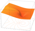
• Plots of the Lambert W function on the complex plane
• 
  z = Re(W₀(x + i y))
• 
  z = Im(W₀(x + i y))
• 
• 

Numerical evaluation

The W function may be approximated using Newton's method, with successive approximations to $w=W(z)$ (so $z=we^{w}$) being

$w_{j+1}=w_{j}-{\frac {w_{j}e^{w_{j}}-z}{e^{w_{j}}+w_{j}e^{w_{j}}}}.$

The W function may also be approximated using Halley's method,

$w_{j+1}=w_{j}-{\frac {w_{j}e^{w_{j}}-z}{e^{w_{j}}(w_{j}+1)-{\frac {(w_{j}+2)(w_{j}e^{w_{j}}-z)}{2w_{j}+2}}}}$

given in Corless et al. to compute W.

Software

The LambertW function is implemented as LambertW in Maple, lambertw in GP (and glambertW in PARI), lambertw in MATLAB, also lambertw in octave with the 'specfun' package, as lambert_w in Maxima, as ProductLog (with a silent alias LambertW) in Mathematica, and as gsl_sf_lambert_W0 and gsl_sf_lambert_Wm1 functions in special functions section of the GNU Scientific Library - GSL.

See also

• Wright Omega function
• Lambert's trinomial equation
• Lagrange inversion theorem
• Experimental mathematics
• Holstein–Herring method
• R=T model
• Ross' π lemma

References

• Corless, R.; Gonnet, G.; Hare, D.; Jeffrey, D.; Knuth, Donald (1996). "On the Lambert W function" (PDF). Advances in Computational Mathematics. 5. Berlin, New York: Springer-Verlag: 329–359. doi:10.1007/BF02124750. ISSN 1019-7168Template:Inconsistent citations{{cite journal}}: CS1 maint: postscript (link)
• Chapeau-Blondeau, F. and Monir, A. (2002). "Evaluation of the Lambert W Function and Application to Generation of Generalized Gaussian Noise With Exponent 1/2" (PDF). IEEE Trans. Signal Processing. 50 (9).{{cite journal}}: CS1 maint: multiple names: authors list (link)
• Francis; et al. (2000). "Quantitative General Theory for Periodic Breathing". Circulation. 102 (18): 2214. {{cite journal}}: Explicit use of et al. in: |author= (help) (Lambert function is used to solve delay-differential dynamics in human disease.)
• Hayes, B. (2005). "Why W?". American Scientist. 93: 104–108.
• Roy, R.; Olver, F. W. J. (2010), "Lambert W function", in Olver, Frank W. J.; Lozier, Daniel M.; Boisvert, Ronald F.; Clark, Charles W. (eds.), NIST Handbook of Mathematical Functions, Cambridge University Press, ISBN 978-0-521-19225-5, MR 2723248.
• Stewart, Seán M. (2005). "A New Elementary Function for Our Curricula?" (PDF). Australian Senior Mathematics Journal. 19 (2). Australian Association of Mathematics Teachers: 8–26. ISSN 0819-4564. ERIC EJ720055. {{cite journal}}: Unknown parameter |layurl= ignored (help)
• Veberic, D., "Having Fun with Lambert W(x) Function" arXiv:1003.1628 (2010); Veberic, D. (2012). "Lambert W function for applications in physics". Computer Physics Communications. 183: 2622–2628. doi:10.1016/j.cpc.2012.07.008.{{cite journal}}: CS1 maint: postscript (link)

External links

• National Institute of Science and Technology Digital Library - Lambert W
• MathWorld - Lambert W-Function
• Computing the Lambert W function
• Corless et al. Notes about Lambert W research
• Extreme Mathematics. Monographs on the Lambert W function, its numerical approximation and generalizations for W-like inverses of transcendental forms with repeated exponential towers.
• GPL C++ implementation with Halley's and Fritsch's iteration.
• Special Functions of the GNU Scientific Library - GSL