
Arithmetic: Difference between revisions
rearranged contents; added sources; adjusted text to match them; added images; some topics covered elsewhere in the article with sources were removed; some overly detailed descriptions were summarized; please let me know if you feel that some essential information was removed so it can be reintegrated into the new version; for earlier drafts, see User:Phlsph7/Arithmetic_operations; for a discussion, see Talk:Arithmetic#Changes_to_the_article Tag: Disambiguation links added |
|||
| Line 76: | Line 76: | ||
Another positional numeral system used extensively in [[computer arithmetic]] is the [[binary system]], which has a radix of 2. This means that the first digit is multiplied by <math>2^0</math>, the next digit by <math>2^1</math>, and so on. For example, the number 13 is written as 1101 in the binary notation, which stands for <math>1 \cdot 2^3 + 1 \cdot 2^2 + 0 \cdot 2^1 + 1 \cdot 2^0</math>. In computing, each digit in the binary notation is corresponds to one [[bit]].{{sfn|Nagel|2002|p=178}}{{sfn|Jena|2021|pp=[https://books.google.com/books?id=qRpSEAAAQBAJ&pg=PA20 20–21]}}{{sfn|Null|Lobur|2006|p=[https://books.google.com/books?id=QGPHAl9GE-IC&pg=PA40 40]}} The earliest positional system was developed by [[Sumer|ancient Sumerians]] and had a radix of 60.{{sfn|Stakhov|2020|p=[https://books.google.com/books?id=Fkn9DwAAQBAJ&pg=PA74 74]}} |
Another positional numeral system used extensively in [[computer arithmetic]] is the [[binary system]], which has a radix of 2. This means that the first digit is multiplied by <math>2^0</math>, the next digit by <math>2^1</math>, and so on. For example, the number 13 is written as 1101 in the binary notation, which stands for <math>1 \cdot 2^3 + 1 \cdot 2^2 + 0 \cdot 2^1 + 1 \cdot 2^0</math>. In computing, each digit in the binary notation is corresponds to one [[bit]].{{sfn|Nagel|2002|p=178}}{{sfn|Jena|2021|pp=[https://books.google.com/books?id=qRpSEAAAQBAJ&pg=PA20 20–21]}}{{sfn|Null|Lobur|2006|p=[https://books.google.com/books?id=QGPHAl9GE-IC&pg=PA40 40]}} The earliest positional system was developed by [[Sumer|ancient Sumerians]] and had a radix of 60.{{sfn|Stakhov|2020|p=[https://books.google.com/books?id=Fkn9DwAAQBAJ&pg=PA74 74]}} |
||
==Arithmetic operations== |
== Arithmetic operations == |
||
Arithmetic operations are ways of combining, transforming, or manipulating numbers. They are [[Function (mathematics)|functions]] that have numbers both as input and output.{{sfn|Nagel|2002|p=179}}{{sfn|Husserl|Willard|2012|pp=[https://books.google.com/books?id=lxftCAAAQBAJ&pg=PR44 XLIV–XLV]|loc=Translator's Introduction}}{{sfn|O'Leary|2015|p=[https://books.google.com/books?id=Ci6kBgAAQBAJ&pg=PA190 190]}} The most important operations in arithmetic are [[addition]], [[subtraction]], [[multiplication]], [[Division (mathematics)|division]], [[exponentiation]], and [[logarithm]].{{sfn|Nagel|2002|p=177}}{{sfn|EoM staff|2020a}}{{sfn|Rising|Matthews|Schoaff|Matthew|2021|p=[https://books.google.com/books?id=hjVZEAAAQBAJ&pg=PA110 110]}}{{sfn|Nagel|2002|pp=179–180}} If these operations are performed on variables rather than numbers, they are sometimes referred to as [[algebraic operations]].{{sfn|Khan|Graham|2018|pp=[https://books.google.com/books?id=vy73DwAAQBAJ&pg=PA9 9–10]}}{{sfn|Smyth|1864|p=[https://books.google.com/books?id=BqQZAAAAYAAJ&pg=PA55 55]}} |
|||
{{See also|Algebraic operation}} |
|||
The basic arithmetic operations are addition, subtraction, multiplication and division, although arithmetic also includes more advanced operations, such as manipulations of [[percentage]]s,<ref name=":2">{{cite web |title=Definition of Arithmetic |url=https://www.mathsisfun.com/definitions/arithmetic.html |website=mathsisfun.com |access-date=2020-08-25 |archive-date=2020-12-31 |archive-url=https://web.archive.org/web/20201231202630/https://www.mathsisfun.com/definitions/arithmetic.html |url-status=live }}</ref> [[square root]]s, [[exponentiation]], [[logarithmic function]]s, and even [[trigonometric function]]s, in the same vein as logarithms ([[prosthaphaeresis]]). Arithmetic expressions must be evaluated according to the intended sequence of operations. There are several methods to specify this, either—most common, together with [[infix notation]]—explicitly using parentheses and relying on [[Order of operations|precedence rules]], or using a [[Polish notation|prefix]] or [[Reverse Polish notation|postfix]] notation, which uniquely fix the order of execution by themselves. Any set of objects upon which all four arithmetic operations (except [[division by zero]]) can be performed, and where these four operations obey the usual laws (including distributivity), is called a [[field mathematics|field]].<ref name=Oxford>{{cite book |last1=Tapson |first1=Frank |year=1996 |title=The Oxford Mathematics Study Dictionary |publisher=Oxford University Press |isbn=0-19-914551-2}}</ref> |
|||
Two important concepts in relation to arithmetic operations are [[identity element]]s and inverse elements. The identity element or neutral element of an operation does not cause any change if it is applied to another element. For example, the identity element of addition is 0 since any sum of a number and 0 results in the same number. The inverse element is the element that results in the identity element when combined with another element. For instance, the [[additive inverse]] of the number 6 is -6 since their sum is 0.{{sfn|Tarasov|2008|pp=[https://books.google.com/books?id=pHK11tfdE3QC&pg=PA57 57–58]}}{{sfn|Mazzola|Milmeister|Weissmann|2004|p=[https://books.google.com/books?id=CkFCCA-2sRgC&pg=PA66 66]}}{{sfn|Krenn|Lorünser|2023|p=[https://books.google.com/books?id=RRi2EAAAQBAJ&pg=PA8 8]}} |
|||
===Addition=== |
|||
{{main|Addition}} |
|||
Addition, denoted by the symbol <math>+</math>, is the most basic operation of arithmetic. In its simple form, addition combines two numbers, the [[addend|''addends'' or ''terms'']], into a single number, the [[summation|''sum'']] of the numbers (such as {{math|2 + 3 {{=}} 5}} or {{math|3 + 5 {{=}} 8}}). |
|||
There are not only inverse elements but also [[inverse function|inverse operations]]. In an informal sense, one operation is the inverse of another operation if it undoes the first operation. For example, subtraction is the inverse of addition since a number returns to its original value if a second number is first added and subsequently subtracted, as in <math>13 + 4 - 4 = 13</math>. Defined more formally, the operation "<math>\star</math>" is an inverse of the operation "<math>\circ</math>" if it fulfills the following condition: <math>t \star s = r</math> if and only if <math>r \circ s = t</math>.{{sfn|Kay|2021|pp=[https://books.google.com/books?id=aw81EAAAQBAJ&pg=PA44 44–45]}}{{sfn|Wright|Ellemor-Collins|Tabor|2011|p=[https://books.google.com/books?id=3yqdEAAAQBAJ&pg=PA136 136]}} |
|||
Adding finitely many numbers can be viewed as repeated simple addition; this procedure is known as [[summation]], a term also used to denote the definition for "adding infinitely many numbers" in an [[series (mathematics)|infinite series]]. Repeated addition of the number [[one|1]] is the most basic form of [[counting]]; the result of adding {{math|1}} is usually called the [[successor function|successor]] of the original number. |
|||
[[Commutativity]] and [[associativity]] are laws governing the order in which some arithmetic operations can be carried out. An operation is commutative if the order of the arguments can be changed without affecting the results. This is the case for addition, for example, <math>7 + 9</math> is the same as <math>9 + 7</math>. Associativity is a rule that affects the order in which a series of operations can be carried out. An operation is associative if in a series of two operations, it does not matter which operation is carried out first. This is the case for multiplication, for example, since <math>(5 \times 4) \times 2</math> is the same as <math>5 \times (4 \times 2)</math>.{{sfn|Krenn|Lorünser|2023|p=[https://books.google.com/books?id=RRi2EAAAQBAJ&pg=PA8 8]}}{{sfn|Mazzola|Milmeister|Weissmann|2004|p=[https://books.google.com/books?id=CkFCCA-2sRgC&pg=PA66 66]}} |
|||
Addition is [[commutative]] and [[associative]], so the order in which finitely many terms are added does not matter. |
|||
=== Addition and subtraction === |
|||
The [[0 (number)|number {{math|0}}]] has the property that, when added to any number, it yields that same number; so, it is the [[identity element]] of addition, or the [[additive identity]]. |
|||
{{main|Addition|Subtraction}} |
|||
{{multiple image |
|||
For every number {{mvar|x}}, there is a number denoted {{math|–''x''}}, called the ''[[opposite (mathematics)|opposite]]'' of {{mvar|x}}, such that {{math|1=''x'' + (–''x'') = 0}} and {{math|1= (–''x'') + ''x'' = 0}}. So, the opposite of {{mvar|x}} is the [[inverse element|inverse]] of {{mvar|x}} with respect to addition, or the [[additive inverse]] of {{mvar|x}}. For example, the opposite of {{math|7}} is {{math|−7}}, since {{math|7 + (−7) {{=}} 0}}. |
|||
|perrow = 1 / 1 |
|||
|total_width = 300 |
|||
|image1 = Addition1.png |
|||
|alt1 = Diagram showing addition |
|||
|link1 = Addition |
|||
|image2 = Subtraction.png |
|||
|alt2 = Diagram showing subtraction |
|||
|link2 = Subtraction |
|||
|footer = Addition and subtraction |
|||
}} |
|||
Addition is an arithmetic operation in which two numbers, called the addends, are combined into a single number, called the sum. The symbol of addition is <math>+</math>. Examples are <math>2 + 2 = 4</math> and <math>6.3 + 1.26 = 7.56</math>.{{sfn|Musser|Peterson|Burger|2013|p=[https://books.google.com/books?id=8jh7DwAAQBAJ&pg=PA87 87]}}{{sfn|Romanowski|2008|p=303}} The term [[summation]] is used if several additions are performed in a row. Counting is a type of repeated addition in which the number 1 is continuously added.{{sfn|Burgin|2022|p=[https://books.google.com/books?id=rWF2EAAAQBAJ&pg=PA25 25]}} |
|||
Addition can also be interpreted geometrically, as in the following example. |
|||
If we have two sticks of lengths ''2'' and ''5'', then, if the sticks are aligned one after the other, the length of the combined stick becomes ''7'', since {{math|2 + 5 {{=}} 7}}. |
|||
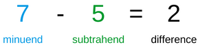
Subtraction is the inverse of addition. In it, one number, known as the subtrahend, is taken away from another, known as the minuend. The result of this operation is called the difference. The symbol of subtraction is <math>-</math>.{{sfn|Romanowski|2008|p=303}}{{sfn|Musser|Peterson|Burger|2013|pp=[https://books.google.com/books?id=8jh7DwAAQBAJ&pg=PA93 93–94]}}{{sfn|Kay|2021|pp=[https://books.google.com/books?id=aw81EAAAQBAJ&pg=PA44 44–45]}}{{sfn|Wright|Ellemor-Collins|Tabor|2011|p=[https://books.google.com/books?id=3yqdEAAAQBAJ&pg=PA136 136]}} Examples are <math>14 - 8 = 6</math> and <math>45 - 1.7 = 43.3</math>. Subtraction is often treated as a special case of addition: instead of subtracting a positive number, it is also possible to add a negative number. For instance <math>14 - 8 = 14 + (-8)</math>. This helps to simplify mathematical computations by reducing the number of basic arithmetic operations needed to perform calculations.{{sfn|Wheater|2015|p=[https://books.google.com/books?id=Q7R3EAAAQBAJ&pg=PP19 19]}}{{sfn|Wright|Ellemor-Collins|Tabor|2011|p=[https://books.google.com/books?id=3yqdEAAAQBAJ&pg=PA136 136–137]}}{{sfn|Achatz|Anderson|2005|p=[https://books.google.com/books?id=YOdtemSmzQQC&pg=PA18 18]}} |
|||
===Subtraction=== |
|||
{{Main|Subtraction}} |
|||
{{See also|Method of complements}} |
|||
Subtraction, denoted by the symbol <math>-</math>, is the inverse operation to addition. Subtraction finds the ''difference'' between two numbers, the ''minuend'' minus the ''subtrahend'': {{math|''D'' {{=}} ''M'' − ''S''.}} Resorting to the previously established addition, this is to say that the difference is the number that, when added to the subtrahend, results in the minuend: {{math|''D'' + ''S'' {{=}} ''M''.}}<ref name=":1">{{cite encyclopedia |title=Arithmetic |url=https://www.britannica.com/science/arithmetic |encyclopedia=[[Encyclopedia Britannica]] |language=en |access-date=2020-08-25 |archive-date=2020-11-12 |archive-url=https://web.archive.org/web/20201112014336/https://www.britannica.com/science/arithmetic |url-status=live }}</ref> |
|||
The additive identity element is 0 and the additive inverse of a number is the negative of that number. For example, <math>13 + 0 = 13</math> and <math>13 + (-13) = 0</math>. Addition is both commutative and associative.{{sfn|Mazzola|Milmeister|Weissmann|2004|p=[https://books.google.com/books?id=CkFCCA-2sRgC&pg=PA66 66]}}{{sfn|Romanowski|2008|p=303}}{{sfn|Nagel|2002|pp=179–180}} |
|||
For positive arguments {{mvar|M}} and {{mvar|S}} holds: |
|||
:If the minuend is larger than the subtrahend, the difference {{mvar|D}} is positive. |
|||
:If the minuend is smaller than the subtrahend, the difference {{mvar|D}} is negative. |
|||
In any case, if minuend and subtrahend are equal, the difference {{math|''D'' {{=}} 0.}} |
|||
=== Multiplication and division === |
|||
Subtraction is neither [[Commutative property|commutative]] nor [[Associative property|associative]]. For that reason, the construction of this inverse operation in modern algebra is often discarded in favor of introducing the concept of inverse elements (as sketched under {{Section link||Addition}}), where subtraction is regarded as adding the additive inverse of the subtrahend to the minuend, that is, {{math|''a'' − ''b'' {{=}} ''a'' + (−''b'')}}. The immediate price of discarding the binary operation of subtraction is the introduction of the (trivial) [[unary operation]], delivering the additive inverse for any given number, and losing the immediate access to the notion of [[difference (mathematics)|difference]], which is potentially misleading when negative arguments are involved. |
|||
{{main|Multiplication|Division (mathematics)}} |
|||
{{multiple image |
|||
For any representation of numbers, there are methods for calculating results, some of which are particularly advantageous in exploiting procedures, existing for one operation, by small alterations also for others. For example, digital computers can reuse existing adding-circuitry and save additional circuits for implementing a subtraction, by employing the method of [[two's complement]] for representing the additive inverses, which is extremely easy to implement in hardware ([[Inverter (logic gate)|negation]]). The trade-off is the halving of the number range for a fixed word length. |
|||
|perrow = 1 / 1 |
|||
|total_width = 300 |
|||
|image1 = Multiplication1.png |
|||
|alt1 = Diagram showing multiplication |
|||
|link1 = Multiplication |
|||
|image2 = Division1.png |
|||
|alt2 = Diagram showing division |
|||
|link2 = Division (mathematics) |
|||
|footer = Multiplication and division |
|||
}} |
|||
Multiplication is an arithmetic operation in which two numbers, called the multiplier and the multiplicant, are combined into a single number called the product.{{sfn|Romanowski|2008|p=303}}{{sfn|Musser|Peterson|Burger|2013|pp=[https://books.google.com/books?id=8jh7DwAAQBAJ&pg=PA101 101–102]}} The symbols of multiplication are <math>\times</math>, <math>\cdot</math>, and *. Examples are <math>2 \times 3 = 6</math> and <math>0.3 \cdot 5 = 1.5</math>. If the multiplicant is a natural number then multiplication is the same as repeated addition, as in <math>2 \times 3 = 2 + 2 + 2</math>.{{sfn|Romanowski|2008|p=304}}{{sfn|Wright|Ellemor-Collins|Tabor|2011|p=[https://books.google.com/books?id=3yqdEAAAQBAJ&pg=PA136 136]}}{{sfn|Musser|Peterson|Burger|2013|pp=[https://books.google.com/books?id=8jh7DwAAQBAJ&pg=PA101 101–102]}} |
|||
A formerly widespread method to achieve a correct change amount, knowing the due and given amounts, is the ''counting up method'', which does not explicitly generate the value of the difference. Suppose an amount ''P'' is given in order to pay the required amount ''Q'', with ''P'' greater than ''Q''. Rather than explicitly performing the subtraction ''P'' − ''Q'' = ''C'' and counting out that amount ''C'' in change, money is counted out starting with the successor of ''Q'', and continuing in the steps of the currency, until ''P'' is reached. Although the amount counted out must equal the result of the subtraction ''P'' − ''Q'', the subtraction was never really done and the value of ''P'' − ''Q'' is not supplied by this method. |
|||
Division is the inverse of multiplication. In it, one number, known as the dividend, is split into several equal parts by another number, known as the divisor. The result of this operation is called the [[quotient]]. The symbols of division are <math>\div</math> and <math>/</math>. Examples are <math>48 \div 8 = 6</math> and <math>29.4 / 1.4 = 21</math>.{{sfn|Romanowski|2008|p=303}}{{sfn|Wheater|2015|p=[https://books.google.com/books?id=Q7R3EAAAQBAJ&pg=PP19 19]}}{{sfn|Wright|Ellemor-Collins|Tabor|2011|p=[https://books.google.com/books?id=3yqdEAAAQBAJ&pg=PA136 136]}} Division is often treated as a special case of multiplication: instead of dividing by a number, it is also possible to multiply by its [[reciprocal]]. The reciprocal of a number is 1 divided by that number. For instance, <math>48 \div 8 = 48 \times \tfrac{1}{8}</math>.{{sfn|Kay|2021|p=[https://books.google.com/books?id=aw81EAAAQBAJ&pg=PA117 117]}}{{sfn|Wheater|2015|p=[https://books.google.com/books?id=Q7R3EAAAQBAJ&pg=PP19 19]}}{{sfn|Wright|Ellemor-Collins|Tabor|2011|p=[https://books.google.com/books?id=3yqdEAAAQBAJ&pg=PA136 136–137]}} |
|||
===Multiplication=== |
|||
{{main|Multiplication}} |
|||
Multiplication, denoted by the symbols <math>\times</math> or <math>\cdot</math>, is the second basic operation of arithmetic. Multiplication also combines two numbers into a single number, the ''product''. The two original numbers are called the ''multiplier'' and the ''multiplicand'', mostly both are called ''factors''. |
|||
The [[multiplicative identity]] element is 1 and the multiplicative inverse of a number is the reciprocal of that number. For example, <math>13 \times 1 = 13</math> and <math>13 \times \tfrac{1}{13} = 1</math>. Multiplication is both commutative and associative.{{sfn|Mazzola|Milmeister|Weissmann|2004|p=[https://books.google.com/books?id=CkFCCA-2sRgC&pg=PA66 66]}}{{sfn|Romanowski|2008|pp=303–304}}{{sfn|Nagel|2002|pp=179–180}} |
|||
Multiplication may be viewed as a scaling operation. If the numbers are imagined as lying in a line, multiplication by a number greater than 1, say ''x'', is the same as stretching everything away from 0 uniformly, in such a way that the number 1 itself is stretched to where ''x'' was. Similarly, multiplying by a number less than 1 can be imagined as squeezing towards 0, in such a way that 1 goes to the multiplicand. |
|||
=== Exponentiation and logarithm === |
|||
Another view on multiplication of integer numbers (extendable to rationals but not very accessible for real numbers) is by considering it as repeated addition. For example. {{math|3 × 4}} corresponds to either adding {{math|3}} times a {{math|4}}, or {{math|4}} times a {{math|3}}, giving the same result. There are different opinions on the advantageousness of these [[Multiplication and repeated addition|paradigmata]] in math education. |
|||
{{main|Exponentiation|Logarithm}} |
|||
{{multiple image |
|||
Multiplication is commutative and associative; further, it is [[distributivity|distributive]] over addition and subtraction. The [[multiplicative identity]] is 1, since multiplying any number by 1 yields that same number. The [[multiplicative inverse]] for any number except {{math|0}} is the [[reciprocal (mathematics)|reciprocal]] of this number, because multiplying the reciprocal of any number by the number itself yields the multiplicative identity {{math|1}}. {{math|0}} is the only number without a multiplicative inverse, and the result of multiplying any number and {{math|0}} is again {{math|0.}} One says that {{math|0}} is not contained in the multiplicative [[Group (mathematics)|group]] of the numbers. |
|||
|perrow = 1 / 1 |
|||
|total_width = 300 |
|||
|image1 = Exponentiation.png |
|||
|alt1 = Diagram showing exponentiation |
|||
|link1 = exponentiation |
|||
|image2 = Logarithm1.png |
|||
|alt2 = Diagram showing logarithm |
|||
|link2 = logarithm |
|||
|footer = Exponentiation and logarithm |
|||
}} |
|||
Exponentiation is an arithmetic operation in which a number, known as the base, is raised to the power of another number, known as the exponent. The result of this operation is called the power. Exponentiation is sometimes expressed using the symbol ^ but the more common way is to write the exponent in [[superscript]] right after the base. Examples are <math>2^4 = 16</math> and <math>3</math>^<math>3 = 27</math>. If the exponent is a natural number then exponentiation is the same as repeated multiplication, as in <math>2^4 = 2 \times 2 \times 2 \times 2</math>.{{sfn|Musser|Peterson|Burger|2013|pp=[https://books.google.com/books?id=8jh7DwAAQBAJ&pg=PA117 117–118]}}{{sfn|Kay|2021|pp=[https://books.google.com/books?id=aw81EAAAQBAJ&pg=PA27 27–28]}} |
|||
The product of ''a'' and ''b'' is written as {{math|''a'' × ''b''}} or {{math|''a''·''b''}}. It can also written by simple juxtaposition: ''ab''. In computer programming languages and software packages (in which one can only use characters normally found on a keyboard), it is often written with an asterisk: <code>a * b</code>. |
|||
Roots are a special type of exponentiation using a [[nth root|fractional exponent]]. For example, the [[square root]] of a number is the same as raising the number to the power of <math>\tfrac{1}{2}</math> and the [[cube root]] of a number is the same as raising the number to the power of <math>\tfrac{1}{3}</math>. Examples are <math>\sqrt{4} = 4^{\tfrac{1}{2}} = 2</math> and <math>\sqrt[3]{27} = 27^{\tfrac{1}{3}} = 3</math>.{{sfn|Kay|2021|p=[https://books.google.com/books?id=aw81EAAAQBAJ&pg=PA118 118]}}{{sfn|Klose|2014|p=[https://books.google.com/books?id=rG7iBQAAQBAJ&pg=PA105 105]}} |
|||
Algorithms implementing the operation of multiplication for various representations of numbers are by far more costly and laborious than those for addition. Those accessible for manual computation either rely on breaking down the factors to single place values and applying repeated addition, or on employing [[Mathematical table|tables]] or [[slide rules]], thereby mapping multiplication to addition and vice versa. These methods are outdated and are gradually replaced by mobile devices. Computers use diverse sophisticated and highly optimized algorithms, to implement multiplication and division for the various number formats supported in their system. |
|||
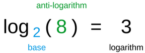
Logarithm is the inverse of exponentiation. In it, the base and the argument of the logarithm are used to determine the power to which the base must be raised to produce the argument. The result of this operation is known as the anti-logarithm. For example, to determine the logarithm of 16 in relation to the base 2, it is necessary to find what exponent should be used on the base 2 for the result to be 16. The anti-logarithm of this operation is 4 since 2 raised by 4 results in 16.{{sfn|Kay|2021|pp=[https://books.google.com/books?id=aw81EAAAQBAJ&pg=PA121 121–122]}}{{sfn|Rodda|Little|2015|p=[https://books.google.com/books?id=cb_dCgAAQBAJ&pg=PA7 7]}} |
|||
===Division=== |
|||
{{main|Division (mathematics)}} |
|||
Division, denoted by the symbols <math>\div</math> or <math>/</math>, is essentially the inverse operation to multiplication. Division finds the ''quotient'' of two numbers, the ''dividend'' divided by the ''divisor''. Under common rules, dividend [[division by zero|divided by zero]] is undefined. For distinct positive numbers, if the dividend is larger than the divisor, the quotient is greater than 1, otherwise it is less than or equal to 1 (a similar rule applies for negative numbers). The quotient multiplied by the divisor always yields the dividend. |
|||
Exponentiation and logarithm do not have general identity elements and inverse elements like addition and multiplication. The neutral element of exponentiation in relation to the exponent is 1, as in <math>14^1 = 14</math>. However, exponentiation does not have a general identity element since 1 is not the neutral element for the base.{{sfn|Kay|2021|p=[https://books.google.com/books?id=aw81EAAAQBAJ&pg=PA117 117]}}{{sfn|Mazzola|Milmeister|Weissmann|2004|p=[https://books.google.com/books?id=CkFCCA-2sRgC&pg=PA66 66]}} Exponentiation and logarithm are neither commutative nor associative.{{sfn|Sally|Sally (Jr.)|2012|p=[https://books.google.com/books?id=Ntjq07-FA_IC&pg=PA3 3]}}{{sfn|Klose|2014|pp=[https://books.google.com/books?id=rG7iBQAAQBAJ&pg=PA107 107–108]}} |
|||
Division is neither commutative nor associative. So as explained in {{Section link||Subtraction}}, the construction of the division in modern algebra is discarded in favor of constructing the inverse elements with respect to multiplication, as introduced in {{Section link||Multiplication}}. Hence division is the multiplication of the dividend with the [[multiplicative inverse|reciprocal]] of the divisor as factors, that is, {{math|''a'' ÷ ''b'' {{=}} ''a'' × {{sfrac|1|''b''}}.}} |
|||
Within the natural numbers, there is also a different but related notion called [[Euclidean division]], which outputs two numbers after "dividing" a natural {{mvar|N}} (numerator) by a natural {{mvar|D}} (denominator): first a natural {{mvar|Q}} (quotient), and second a natural {{mvar|R}} (remainder) such that {{math|''N'' {{=}} ''D''×''Q'' + ''R''}} and {{math|0 ≤ ''R'' < ''Q''.}} |
|||
In some contexts, including computer programming and advanced arithmetic, division is extended with another output for the remainder. This is often treated as a separate operation, the [[Modulo operation]], denoted by the symbol <math>%</math> or the word <math>mod</math>, though sometimes a second output for one "divmod" operation.<ref>{{cite web |title=Python divmod() Function |url=https://www.w3schools.com/python/ref_func_divmod.asp |website=W3Schools |publisher=Refsnes Data |access-date=2021-03-13 |archive-date=2021-03-13 |archive-url=https://web.archive.org/web/20210313103613/https://www.w3schools.com/python/ref_func_divmod.asp |url-status=live }}</ref> In either case, [[Modular arithmetic]] has a variety of use cases. Different implementations of division (floored, truncated, Euclidean, etc.) correspond with different implementations of modulus. |
|||
== Integer arithmetic == |
== Integer arithmetic == |
||
| Line 467: | Line 482: | ||
* {{cite book |last1=Nagel |first1=Rob |title=U-X-L Encyclopedia of Science |date=2002 |publisher=U-X-L |isbn=978-0-7876-5440-5 |url=https://www.encyclopedia.com/science-and-technology/mathematics/mathematics/arithmetic |language=en}} |
* {{cite book |last1=Nagel |first1=Rob |title=U-X-L Encyclopedia of Science |date=2002 |publisher=U-X-L |isbn=978-0-7876-5440-5 |url=https://www.encyclopedia.com/science-and-technology/mathematics/mathematics/arithmetic |language=en}} |
||
* {{cite web |last1=Hosch |first1=William L. |title=Rational number |url=https://www.britannica.com/science/rational-number |website=Encyclopædia Britannica |access-date=24 October 2023 |language=en |date=2023}} |
* {{cite web |last1=Hosch |first1=William L. |title=Rational number |url=https://www.britannica.com/science/rational-number |website=Encyclopædia Britannica |access-date=24 October 2023 |language=en |date=2023}} |
||
* {{cite book |last1=Smyth |first1=William |title=Elementary Algebra: For Schools and Academies |date=1864 |publisher=Bailey and Noyes |url=https://books.google.com/books?id=BqQZAAAAYAAJ&pg=PA55 |language=en}} |
|||
* {{cite book |last1=Husserl |first1=Edmund |last2=Willard |first2=Dallas |title=Philosophy of Arithmetic: Psychological and Logical Investigations with Supplementary Texts from 1887–1901 |date=6 December 2012 |publisher=Springer Science & Business Media |isbn=978-94-010-0060-4 |url=https://books.google.com/books?id=lxftCAAAQBAJ&pg=PR44 |language=en |chapter=Translator's Introduction}} |
|||
* {{cite book |last1=O'Leary |first1=Michael L. |title=A First Course in Mathematical Logic and Set Theory |date=8 September 2015 |publisher=John Wiley & Sons |isbn=978-0-470-90588-3 |url=https://books.google.com/books?id=Ci6kBgAAQBAJ&pg=PA190 |language=en}} |
|||
* {{cite book |last1=Khan |first1=Khalid |last2=Graham |first2=Tony Lee |title=Engineering Mathematics with Applications to Fire Engineering |date=12 June 2018 |publisher=CRC Press |isbn=978-1-351-59761-6 |url=https://books.google.com/books?id=vy73DwAAQBAJ&pg=PA9 |language=en}} |
|||
* {{cite book |last1=Rising |first1=Gerald R. |last2=Matthews |first2=James R. |last3=Schoaff |first3=Eileen |last4=Matthew |first4=Judith |title=About Mathematics |date=2021 |publisher=Linus Learning |isbn=978-1-60797-892-3 |url=https://books.google.com/books?id=hjVZEAAAQBAJ&pg=PA110 |language=en}} |
|||
* {{cite book |last1=Kay |first1=Anthony |title=Number Systems: A Path into Rigorous Mathematics |date=14 September 2021 |publisher=CRC Press |isbn=978-0-429-60776-9 |url=https://books.google.com/books?id=aw81EAAAQBAJ&pg=PA117 |language=en}} |
|||
* {{cite book |last1=Tarasov |first1=Vasily |title=Quantum Mechanics of Non-Hamiltonian and Dissipative Systems |date=6 June 2008 |publisher=Elsevier |isbn=978-0-08-055971-1 |url=https://books.google.com/books?id=pHK11tfdE3QC&pg=PA57 |language=en}} |
|||
* {{cite book |last1=Mazzola |first1=Guerino |last2=Milmeister |first2=Gérard |last3=Weissmann |first3=Jody |title=Comprehensive Mathematics For Computer Scientists 1: Sets And Numbers, Graphs And Algebra, Logic And Machines, Linear Geometry |date=2004 |publisher=Springer Science & Business Media |isbn=978-3-540-20835-8 |url=https://books.google.com/books?id=CkFCCA-2sRgC&pg=PA66 |language=en}} |
|||
* {{cite book |last1=Krenn |first1=Stephan |last2=Lorünser |first2=Thomas |title=An Introduction to Secret Sharing: A Systematic Overview and Guide for Protocol Selection |date=28 March 2023 |publisher=Springer Nature |isbn=978-3-031-28161-7 |url=https://books.google.com/books?id=RRi2EAAAQBAJ&pg=PA8 |language=en}} |
|||
* {{cite book |last1=Sally |first1=Judith D. |last2=Sally (Jr.) |first2=Paul J. |title=Integers, Fractions, and Arithmetic: A Guide for Teachers |date=2012 |publisher=American Mathematical Soc. |isbn=978-0-8218-8798-1 |url=https://books.google.com/books?id=Ntjq07-FA_IC&pg=PA3 |language=en}} |
|||
* {{cite book |last1=Burgin |first1=Mark |title=Trilogy Of Numbers And Arithmetic - Book 1: History Of Numbers And Arithmetic: An Information Perspective |date=22 April 2022 |publisher=World Scientific |isbn=978-981-12-3685-3 |url=https://books.google.com/books?id=rWF2EAAAQBAJ&pg=PA25 |language=en}} |
|||
* {{cite book |last1=Wheater |first1=Carolyn |title=Algebra I |date=2 June 2015 |publisher=Dorling Kindersley Limited |isbn=978-0-241-88779-0 |url=https://books.google.com/books?id=Q7R3EAAAQBAJ&pg=PP19 |language=en}} |
|||
* {{cite book |last1=Wright |first1=Robert J. |last2=Ellemor-Collins |first2=David |last3=Tabor |first3=Pamela D. |title=Developing Number Knowledge: Assessment,Teaching and Intervention with 7-11 year olds |date=4 November 2011 |publisher=SAGE |isbn=978-1-4462-8927-3 |url=https://books.google.com/books?id=3yqdEAAAQBAJ&pg=PA136 |language=en}} |
|||
* {{cite book |last1=Achatz |first1=Thomas |last2=Anderson |first2=John G. |title=Technical Shop Mathematics |date=2005 |publisher=Industrial Press Inc. |isbn=978-0-8311-3086-2 |url=https://books.google.com/books?id=YOdtemSmzQQC&pg=PA18 |language=en}} |
|||
* {{cite book |last1=Klose |first1=Orval M. |title=The Number Systems and Operations of Arithmetic: An Explanation of the Fundamental Principles of Mathematics Which Underlie the Understanding and Use of Arithmetic, Designed for In-Service Training of Elementary School Teachers Candidates Service Training of Elementary School Teacher Candidates |date=16 May 2014 |publisher=Elsevier |isbn=978-1-4831-3709-4 |url=https://books.google.com/books?id=rG7iBQAAQBAJ&pg=PA107 |language=en}} |
|||
* {{cite book |last1=Rodda |first1=Harvey J. E. |last2=Little |first2=Max A. |title=Understanding Mathematical and Statistical Techniques in Hydrology: An Examples-based Approach |date=2 November 2015 |publisher=John Wiley & Sons |isbn=978-1-119-07659-9 |url=https://books.google.com/books?id=cb_dCgAAQBAJ&pg=PA7 |language=en}} |
|||
==Further reading== |
==Further reading== |
||
Revision as of 13:21, 15 November 2023

Arithmetic (from Ancient Greek ἀριθμός (arithmós) 'number', and τική [τέχνη] (tikḗ [tékhnē]) 'art, craft') is an elementary part of mathematics that consists of the study of the properties of the traditional operations on numbers—addition, subtraction, multiplication, division, exponentiation, and extraction of roots. In the 19th century, Italian mathematician Giuseppe Peano formalized arithmetic with his Peano axioms,[disputed ] which are highly important to the field of mathematical logic today.
History
The prehistory of arithmetic is limited to a small number of artifacts that may indicate the conception of addition and subtraction; the best-known is the Ishango bone from central Africa, dating from somewhere between 20,000 and 18,000 BC, although its interpretation is disputed.[1]
The earliest written records indicate the Egyptians and Babylonians used all the elementary arithmetic operations: addition, subtraction, multiplication, and division, as early as 2000 BC. These artifacts do not always reveal the specific process used for solving problems, but the characteristics of the particular numeral system strongly influence the complexity of the methods. The hieroglyphic system for Egyptian numerals, like the later Roman numerals, descended from tally marks used for counting. In both cases, this origin resulted in values that used a decimal base but did not include positional notation. Complex calculations with Roman numerals required the assistance of a counting board (or the Roman abacus) to obtain the results.
Early number systems that included positional notation were not decimal; these include the sexagesimal (base 60) system for Babylonian numerals and the vigesimal (base 20) system that defined Maya numerals. Because of the place-value concept, the ability to reuse the same digits for different values contributed to simpler and more efficient methods of calculation.
The continuous historical development of modern arithmetic starts with the Hellenistic period of ancient Greece; it originated much later than the Babylonian and Egyptian examples. Prior to the works of Euclid around 300 BC, Greek studies in mathematics overlapped with philosophical and mystical beliefs. Nicomachus is an example of this viewpoint, using the earlier Pythagorean approach to numbers and their relationships to each other in his work, Introduction to Arithmetic.
Greek numerals were used by Archimedes, Diophantus, and others in a positional notation not very different from modern notation. The ancient Greeks lacked a symbol for zero until the Hellenistic period, and they used three separate sets of symbols as digits: one set for the units place, one for the tens place, and one for the hundreds. For the thousands place, they would reuse the symbols for the units place, and so on. Their addition algorithm was identical to the modern method, and their multiplication algorithm was only slightly different. Their long division algorithm was the same, and the digit-by-digit square root algorithm, popularly used as recently as the 20th century, was known to Archimedes (who may have invented it). He preferred it to Hero's method of successive approximation because, once computed, a digit does not change, and the square roots of perfect squares, such as 7485696, terminate immediately as 2736. For numbers with a fractional part, such as 546.934, they used negative powers of 60 instead of negative powers of 10 for the fractional part 0.934.[2]
The ancient Chinese had advanced arithmetic studies dating from the Shang Dynasty and continuing through the Tang Dynasty, from basic numbers to advanced algebra. The ancient Chinese used a positional notation similar to that of the Greeks. Since they also lacked a symbol for zero, they had one set of symbols for the units place and a second set for the tens place. For the hundreds place, they then reused the symbols for the units place, and so on. Their symbols were based on ancient counting rods. The exact time when the Chinese started calculating with positional representation is unknown, though it is known that the adoption started before 400 BC.[3] The ancient Chinese were the first to meaningfully discover, understand, and apply negative numbers. This is explained in the Nine Chapters on the Mathematical Art (Jiuzhang Suanshu), which was written by Liu Hui and dates back to the 2nd century BC.
The gradual development of the Hindu–Arabic numeral system independently devised the place-value concept and positional notation, which combined the simpler methods for computations with a decimal base and the use of a digit representing 0. This allowed the system to consistently represent both large and small integers—an approach that eventually replaced all other systems. In the early 6th century AD, the Indian mathematician Aryabhata incorporated an existing version of this system into his work and experimented with different notations. In the 7th century, Brahmagupta established the use of 0 as a separate number and determined the results for multiplication, division, addition, and subtraction of zero and all other numbers—except for the result of division by zero. His contemporary, the Syriac bishop Severus Sebokht (650 AD) said, "Indians possess a method of calculation that no word can praise enough. Their rational system of mathematics, or of their method of calculation. I mean the system using nine symbols."[4] The Arabs also learned this new method and called it hesab.

Although the Codex Vigilanus described an early form of Arabic numerals (omitting 0) by 976 AD, Leonardo of Pisa (Fibonacci) was primarily responsible for spreading their use throughout Europe after the publication of his book Liber Abaci in 1202. He wrote, "The method of the Indians (Latin Modus Indorum) surpasses any known method to compute. It's a marvelous method. They do their computations using nine figures and symbol zero".[5]
In the Middle Ages, arithmetic was one of the seven liberal arts taught in universities.
The flourishing of algebra in the medieval Islamic world, and also in Renaissance Europe, was an outgrowth of the enormous simplification of computation through decimal notation.
Various types of tools have been invented and widely used to assist in numeric calculations. Before Renaissance, they were various types of abaci. More recent examples include slide rules, nomograms and mechanical calculators, such as Pascal's calculator. At present, they have been supplanted by electronic calculators and computers.
Arithmetic is the fundamental branch of mathematics that studies numbers and their operations. In particular, it deals with numerical calculations using the arithmetic operations of addition, subtraction, multiplication, division, exponentiation, and logarithm.[6][7][8][9] The term "arithmetic" has its root in the Latin term "arithmetica" which derives from the Ancient Greek words ἀριθμός (arithmos), meaning "number", and ἀριθμητική τέχνη (arithmetike tekhne), meaning "the art of counting".[10][11][12]
There are disagreements about its precise definition. According to a narrow characterization, arithmetic deals only with natural numbers.[13][14] However, the more common view is to include operations on integers, rational numbers, real numbers, and sometimes also complex numbers in its scope.[6][7][8][9] Some definitions restrict arithmetic to the field of numerical calculations.[15] When understood in a wider sense, it also includes the study of how the concept of numbers developed, the analysis of properties of and relations between numbers, and the examination of the axiomatic structure of arithmetic operations.[9][16][17]
Arithmetic is closely related to number theory and some authors use the terms as synonyms.[18][19] However, in a more specific sense, number theory is restricted to the study of integers and focuses on their properties and relationships such as divisibility, factorization, and primality.[20][21][22][23] Traditionally, it is known as higher arithmetic.[24][23] Arithmetic is intimately connected to many branches of mathematics that depend on numerical operations. Algebra relies on arithmetic principles to solve equations using variables. These principles also play a key role in calculus in its attempt to determine rates of change and areas under curves. Geometry uses arithmetic operations to measure the properties of shapes while statistics utilizes them to analyze numerical data.[25][26][27][28]
Numbers
Numbers are mathematical objects used to count quantities and measure magnitudes. They are fundamental elements in arithmetic since all arithmetic operations are performed on numbers. There are different types of numbers and different numeral systems to represent them.[29][30][31]
Types

The main types of numbers employed in arithmetic are natural numbers, whole numbers, integers, rational numbers, and real numbers.[32][33][30] The natural numbers are whole numbers that start from 1 and go to infinity. They exclude 0 and negative numbers. They are also known as counting numbers and can be expressed as {1, 2, 3, 4, ...}. The symbol of the natural numbers is . The whole numbers are identical to the natural numbers with the only difference being that they include 0. They can be represented as {0, 1, 2, 3, 4, ...} and have the symbol .[34][32][35][36] Some mathematicians do not draw the distinction between the natural and the whole numbers by including 0 in the set of natural numbers.[37][38] The set of integers encompasses both positive and negative whole numbers. It has the symbol and can be expressed as {..., -2, -1, 0, 1, 2, ...}.[34][32][35][39]


A number is rational if it can be represented as the ratio of two integers. For example, the rational number is formed by dividing the integer 1, called the numerator, by the integer 2, called the denominator. Other examples are and . The set of rational numbers includes all integers, which are fractions with a denominator of 1. The symbol of the rational numbers is .[34][32][35][40] Decimal fractions like 0.3 and 25.12 are a special type of rational numbers since their denominator is a power of 10. For example, 0.3 is equal to , and 25.12 is equal to .[41][42] Every rational number corresponds to a finite or a repeating decimal.[43]


Irrational numbers are numbers that cannot be expressed through the ratio of two integers. Examples are many square roots, such as , and numbers like π and e (Euler's number).[34][32][35] The decimal representation of an irrational number is infinite without repeating decimals.[44][45] The set of rational numbers together with the set of irrational numbers makes up the set of real numbers. The symbol of the real numbers is .[34][35] Even wider classes of numbers include complex numbers and quaternions.[35][46]


Based on how numbers are used, they can be distinguished into cardinal and ordinal numbers. Cardinal numbers, like one, two, and three, are numbers that express the quantity of objects. They answer the question "how many?". Ordinal numbers, such as first, second, and third, indicate order or placement in a series. They answer the question "what position?".[47][48]
Numeral systems
A numeral is a symbol to represent a number and numeral systems are representational frameworks.[49][50][51] They usually have a limited amount of basic numerals, which directly refer to certain numbers. The system governs how these basic numerals may be combined to express any number.[52][53] Numeral systems are either positional or non-positional. All early numeral systems were non-positional.[54][55][56] For non-positional numeral systems, the value of a digit does not depend on its position in the numeral.[55][56]

The simplest non-positional system is the unary numeral system. It relies on one symbol for the number 1. All higher numbers are written by repeating this symbol. For example, the number 7 can be represented by repeating the symbol for 1 seven times. This system makes it cumbersome to write large numbers, which is why many non-positional systems include additional symbols to directly represent larger numbers.[52][57][58] Variations of the unary numeral systems are employed in tally sticks using dents and in tally marks.[59][60]
.png)
Egyptian hieroglyphics had a more complex non-positional numeral system. They have additional symbols for numbers like 10, 100, 1000, and 10,000. These symbols can be combined into a sum to more conveniently express larger numbers. For example, the numeral for 10,405 uses one time the symbol for 10,000, four times the symbol for 100, and five times the symbol for 1. A similar well-known framework is the Roman numeral system. It has the symbols I, V, X, L, C, D, M as its basic numerals to represent the numbers 1, 5, 10, 50, 100, 500, and 1000.[52][57][61]
A numeral system is positional if the position of a basic numeral in a compound expression determines its value. Positional numeral systems have a radix that acts as a multiplier of the different positions. For each subsequent position, the radix is raised to a higher power. In the common decimal system, also called the Hindu–Arabic numeral system, the radix is 10. This means that the first digit is multiplied by , the next digit is multiplied by , and so on. For example, the decimal numeral 532 stands for . Because of the effect of the digits' positions, the numeral 532 differs from the numerals 325 and 253 even though they have the same digits.[62][63][64][65][56]


Another positional numeral system used extensively in computer arithmetic is the binary system, which has a radix of 2. This means that the first digit is multiplied by , the next digit by , and so on. For example, the number 13 is written as 1101 in the binary notation, which stands for . In computing, each digit in the binary notation is corresponds to one bit.[66][67][68] The earliest positional system was developed by ancient Sumerians and had a radix of 60.[69]


Arithmetic operations
Arithmetic operations are ways of combining, transforming, or manipulating numbers. They are functions that have numbers both as input and output.[70][71][72] The most important operations in arithmetic are addition, subtraction, multiplication, division, exponentiation, and logarithm.[73][9][74][75] If these operations are performed on variables rather than numbers, they are sometimes referred to as algebraic operations.[76][77]
Two important concepts in relation to arithmetic operations are identity elements and inverse elements. The identity element or neutral element of an operation does not cause any change if it is applied to another element. For example, the identity element of addition is 0 since any sum of a number and 0 results in the same number. The inverse element is the element that results in the identity element when combined with another element. For instance, the additive inverse of the number 6 is -6 since their sum is 0.[78][79][80]
There are not only inverse elements but also inverse operations. In an informal sense, one operation is the inverse of another operation if it undoes the first operation. For example, subtraction is the inverse of addition since a number returns to its original value if a second number is first added and subsequently subtracted, as in . Defined more formally, the operation "" is an inverse of the operation "" if it fulfills the following condition: if and only if .[81][82]


Commutativity and associativity are laws governing the order in which some arithmetic operations can be carried out. An operation is commutative if the order of the arguments can be changed without affecting the results. This is the case for addition, for example, is the same as . Associativity is a rule that affects the order in which a series of operations can be carried out. An operation is associative if in a series of two operations, it does not matter which operation is carried out first. This is the case for multiplication, for example, since is the same as .[80][79]


Addition and subtraction

Addition is an arithmetic operation in which two numbers, called the addends, are combined into a single number, called the sum. The symbol of addition is . Examples are and .[83][62] The term summation is used if several additions are performed in a row. Counting is a type of repeated addition in which the number 1 is continuously added.[84]


Subtraction is the inverse of addition. In it, one number, known as the subtrahend, is taken away from another, known as the minuend. The result of this operation is called the difference. The symbol of subtraction is .[62][85][81][82] Examples are and . Subtraction is often treated as a special case of addition: instead of subtracting a positive number, it is also possible to add a negative number. For instance . This helps to simplify mathematical computations by reducing the number of basic arithmetic operations needed to perform calculations.[86][87][88]


The additive identity element is 0 and the additive inverse of a number is the negative of that number. For example, and . Addition is both commutative and associative.[79][62][75]


Multiplication and division


Multiplication is an arithmetic operation in which two numbers, called the multiplier and the multiplicant, are combined into a single number called the product.[62][89] The symbols of multiplication are , , and *. Examples are and . If the multiplicant is a natural number then multiplication is the same as repeated addition, as in .[34][82][89]


Division is the inverse of multiplication. In it, one number, known as the dividend, is split into several equal parts by another number, known as the divisor. The result of this operation is called the quotient. The symbols of division are and . Examples are and .[62][86][82] Division is often treated as a special case of multiplication: instead of dividing by a number, it is also possible to multiply by its reciprocal. The reciprocal of a number is 1 divided by that number. For instance, .[90][86][87]


The multiplicative identity element is 1 and the multiplicative inverse of a number is the reciprocal of that number. For example, and . Multiplication is both commutative and associative.[79][17][75]


Exponentiation and logarithm

Exponentiation is an arithmetic operation in which a number, known as the base, is raised to the power of another number, known as the exponent. The result of this operation is called the power. Exponentiation is sometimes expressed using the symbol ^ but the more common way is to write the exponent in superscript right after the base. Examples are and ^. If the exponent is a natural number then exponentiation is the same as repeated multiplication, as in .[91][92]


Roots are a special type of exponentiation using a fractional exponent. For example, the square root of a number is the same as raising the number to the power of and the cube root of a number is the same as raising the number to the power of . Examples are and .[93][94]


![{\displaystyle {\sqrt[{3}]{27}}=27^{\tfrac {1}{3}}=3}](https://wikimedia.org/api/rest_v1/media/math/render/svg/3f1ae94535b4cb79ea265ed5f47ddf85de5e48ed)
Logarithm is the inverse of exponentiation. In it, the base and the argument of the logarithm are used to determine the power to which the base must be raised to produce the argument. The result of this operation is known as the anti-logarithm. For example, to determine the logarithm of 16 in relation to the base 2, it is necessary to find what exponent should be used on the base 2 for the result to be 16. The anti-logarithm of this operation is 4 since 2 raised by 4 results in 16.[95][96]
Exponentiation and logarithm do not have general identity elements and inverse elements like addition and multiplication. The neutral element of exponentiation in relation to the exponent is 1, as in . However, exponentiation does not have a general identity element since 1 is not the neutral element for the base.[90][79] Exponentiation and logarithm are neither commutative nor associative.[97][98]

Integer arithmetic
Integer arithmetic is the branch of arithmetic that deals with the manipulation of positive and negative whole numbers.[34][35][39] Simple one-digit operations can be performed by following or memorizing a table that presents the results of all possible combinations, like an addition table or a multiplication table. Other common methods are verbal counting and finger-counting.[99][100][101]
| + | 0 | 1 | 2 | 3 | 4 | ... |
|---|---|---|---|---|---|---|
| 0 | 0 | 1 | 2 | 3 | 4 | ... |
| 1 | 1 | 2 | 3 | 4 | 5 | ... |
| 2 | 2 | 3 | 4 | 5 | 6 | ... |
| 3 | 3 | 4 | 5 | 6 | 7 | ... |
| 4 | 4 | 5 | 6 | 7 | 8 | ... |
| ... | ... | ... | ... | ... | ... | ... |
| × | 0 | 1 | 2 | 3 | 4 | ... |
|---|---|---|---|---|---|---|
| 0 | 0 | 0 | 0 | 0 | 0 | ... |
| 1 | 0 | 1 | 2 | 3 | 4 | ... |
| 2 | 0 | 2 | 4 | 6 | 8 | ... |
| 3 | 0 | 3 | 6 | 9 | 12 | ... |
| 4 | 0 | 4 | 8 | 12 | 16 | ... |
| ... | ... | ... | ... | ... | ... | ... |

For operations on numbers with more than one digit, different techniques can be employed to calculate the result by using several one-digit operations in a row. For example, in the method addition with carries, the two numbers are written one above the other. Starting from the rightmost digit, each pair of digits is added together. The rightmost digit of the sum is written below them. If the sum is a two-digit number then the leftmost digit, called the "carry", is added to the next pair of digits to the left. This process is repeated until all digits have been added.[102][103] Other methods used for integer additions are the number line method, the partial sum method, and the compensation method.[104][105] A similar technique is used for subtraction: it also starts with the rightmost digit and uses a "borrow" or a negative carry for the column on the left if the result of the one-digit subtraction is negative.[106]

A basic technique of integer multiplication uses repeated addition. For example, the product of 3 × 4 can be calculated as 3 + 3 + 3 + 3.[107] A common technique for multiplication with larger numbers is called long multiplication. This method starts by writing the multiplicand above the multiplier. The calculation begins by multiplying the multiplicand only with the rightmost digit of the multiplier and writing the result below, starting in the rightmost column. The same is done for each digit of the multiplier and the result in each case is shifted one position to the left. As a final step, all the individual products are added to arrive at the total product of the two multi-digit numbers.[108][109] Other techniques used for multiplication are the grid method and the lattice method.[110] Computer science is interested in multiplication algorithms with a low computational complexity to be able to efficiently multiply very large integers, such as the Karatsuba algorithm, the Schönhage-Strassen algorithm, and the Toom-Cook algorithm.[111][112] A common technique used for division is called long division. Other methods include short division and chunking.[113]
Integer arithmetic is not closed under division. This means that when dividing one integer by another integer, the result is not always an integer. For example, 7 divided by 2 is not a whole number but 3.5.[114] One way to ensure that the result is an integer is to round the result to a whole number. However, this method leads to inaccuracies as the original value is altered.[115] Another method is to perform the division only partially and retain the remainder. For example, 7 divided by 2 is 3 with a remainder of 1. These difficulties are avoided by rational arithmetic, which allows for the exact representation of fractions.[116]
A simple method to calculate exponentiation is by repeated multiplication. For example, the exponentiation of 34 can be calculated as 3 × 3 × 3 × 3.[117] A more efficient technique used for large exponents is exponentiation by squaring. It breaks down the calculation into a number of squaring operations. For example, the exponentiation 365 can be written as (((((32)2)2)2)2)2 × 3. By taking advantage of repeated squaring operations, only 7 individual operations are needed rather than the 64 operations required for regular repeated multiplication.[118][119] Methods to calculate logarithms include the Taylor series and continued fractions.[120][121] Integer arithmetic is not closed under logarithm and under exponentiation with negative exponents, meaning that the result of these operations is not always an integer.[122][120]
Rational arithmetic
Rational arithmetic is the branch of arithmetic that deals with the manipulation of numbers that can be expressed as a ratio of two integers.[123][34][35][40] Most arithmetic operations on rational numbers can be calculated by performing a series of integer arithmetic operations on the numerators and the denominators of the involved numbers. If two rational numbers have the same denominator then they can be added by adding their numerators and keeping the common denominator. For example, . A similar procedure is used for subtraction. If the two numbers do not have the same denominator then they must be transformed to find a common denominator. This can be achieved by scaling the first number with the denominator of the second number while scaling the second number with the denominator of the first number. For example, .[124][125]


Two rational numbers are multiplied by multiplying their numerators and their denominators respectively, as in . Dividing one rational number by another can be achieved by multiplying the first number with the reciprocal of the second number. This means that the numerator and the denominator of the second number change position. For example, .[126] Unlike integer arithmetic, rational arithmetic is closed under division as long as the divisor is not 0.[42]


Both integer arithmetic and rational arithmetic are not closed under exponentiation and logarithm.[127] One way to calculate exponentiation with a fractional exponent is to perform two separate calculations: one exponentiation using the numerator of the exponent followed by drawing the nth root of the result based on the denominator of the exponent. For example, . The first operation can be completed using methods like repeated multiplication or exponentiation by squaring. One way to get an approximate result for the second operation is to employ Newton's method, which uses a series of steps to gradually refine an initial guess until it reaches the desired level of accuracy.[128][129][130] The Taylor series or the continued fraction method can be used to calculate logarithms.[120][121]
![{\displaystyle 5^{\tfrac {2}{3}}={\sqrt[{3}]{5^{2}}}}](https://wikimedia.org/api/rest_v1/media/math/render/svg/147336e8a106c1535ff774fd5c724afea1ef4957)
The decimal fraction notation is a special way of representing rational numbers whose denominator is a power of 10. For example, the rational numbers , , and are written as 0.1, 3.71, and 0.0044 in the decimal fraction notation.[42][131] Modified versions of integer calculation methods like addition with carry and long multiplication can be applied to calculations with decimal fractions.[132][133] Not all rational numbers have an finite representation in the decimal notation. For example, the rational number corresponds 0.333... with an infinite number of 3s. The shortened notation for this type of repeating decimal is 0.3.[134][131] Every repeating decimal expresses a rational number.[43]


Real arithmetic
Real arithmetic is the branch of arithmetic that deals with the manipulation of both rational and irrational numbers. Irrational numbers are numbers that cannot be expressed through fractions or repeated decimals, like the root of 2 and π.[44][135][45][136] Unlike rational arithmetic, real arithmetic is closed under exponentiation as long as it uses a positive number as its base. The same is true for the logarithm of positive real numbers as long as the logarithm base is positive and not 1.[137][138][139]
Irrational numbers involve an infinite non-repeating series of decimal digits. Because of this, there is often no simple and accurate way to express the results of arithmetic operations like or . [44][135][45][136] In cases where absolute precision is not required, the problem of calculating arithmetic operations on real numbers is usually addressed by truncation or rounding. For truncation, a certain number of significant digits to the left are kept and additional digits to the right of the last significant digit are removed. For example, the number π has an infinite number of digits starting with 3.14159... . If this number is truncated to 4 significant digits, the result is 3.141. Rounding is a similar process in which the last significant digit is increased by one if the next digit is 5 or greater. If the next digit is less than 5, the last digit remains the same. For example, if the number π is rounded to 4 significant digits, the result is 3.142 because the following digit is a 5.[140][141][142] These methods are essential to allow computers to efficiently perform calculations on real numbers.[143]


Very large and very small real numbers are often expressed using normalized scientific notation. In it, numbers are represented using a so-called significand multiplied by a power of 10. The significand is a digit followed by a decimal point and a series of digits. For example, the normalized scientific notation of the number 8276000 is and the number 0.00735 has the normalized scientific notation of .[144][145]


A common method employed by computers to approximate real arithmetic is called floating-point arithmetic. It represents real numbers similar to the scientific notation through three numbers: a significand, a base, and an exponent.[146] The precision of the significand is limited by the number of bits allocated to represent it. If an arithmetic operation results in a number that requires more bits than are available, the computer rounds the result to the closest representable number. This leads to rounding errors.[143][146][147] A consequence of this behavior is that certain laws of arithmetic are violated by floating-point arithmetic. For example, floating-point addition is not associative since the rounding errors introduced can depend on the order of the additions. This means that the result of is sometimes different from the result of .[148][149] The most common technical standard used for floating-point arithmetic is called IEEE 754. Among other things, it determines how numbers are represented, how arithmetic operations and rounding are performed, and how errors and exceptions are handled.[150][151][152]


Fundamental theorem of arithmetic
The fundamental theorem of arithmetic states that any integer greater than 1 has a unique prime factorization (a representation of a number as the product of prime factors), excluding the order of the factors. For example, 252 only has one prime factorization:
- 252 = 22 × 32 × 71
Euclid's Elements first introduced this theorem, and gave a partial proof (which is called Euclid's lemma). The fundamental theorem of arithmetic was first proven by Carl Friedrich Gauss.
The fundamental theorem of arithmetic is one of the reasons why 1 is not considered a prime number. Other reasons include the sieve of Eratosthenes, and the definition of a prime number itself (a natural number greater than 1 that cannot be formed by multiplying two smaller natural numbers.).
Decimal arithmetic
Decimal representation refers exclusively, in common use, to the written numeral system employing arabic numerals as the digits for a radix 10 ("decimal") positional notation; however, any numeral system based on powers of 10, e.g., Greek, Cyrillic, Roman, or Chinese numerals may conceptually be described as "decimal notation" or "decimal representation".
Modern methods for four fundamental operations (addition, subtraction, multiplication and division) were first devised by Brahmagupta of India. This was known during medieval Europe as "Modus Indorum" or Method of the Indians. Positional notation (also known as "place-value notation") refers to the representation or encoding of numbers using the same symbol for the different orders of magnitude (e.g., the "ones place", "tens place", "hundreds place") and, with a radix point, using those same symbols to represent fractions (e.g., the "tenths place", "hundredths place"). For example, 507.36 denotes 5 hundreds (102), plus 0 tens (101), plus 7 units (100), plus 3 tenths (10−1) plus 6 hundredths (10−2).
The concept of 0 as a number comparable to the other basic digits is essential to this notation, as is the concept of 0's use as a placeholder, and as is the definition of multiplication and addition with 0. The use of 0 as a placeholder and, therefore, the use of a positional notation is first attested to in the Jain text from India entitled the Lokavibhâga, dated 458 AD and it was only in the early 13th century that these concepts, transmitted via the scholarship of the Arabic world, were introduced into Europe by Fibonacci[153] using the Hindu–Arabic numeral system.
Algorism comprises all of the rules for performing arithmetic computations using this type of written numeral. For example, addition produces the sum of two arbitrary numbers. The result is calculated by the repeated addition of single digits from each number that occupies the same position, proceeding from right to left. An addition table with ten rows and ten columns displays all possible values for each sum. If an individual sum exceeds the value 9, the result is represented with two digits. The rightmost digit is the value for the current position, and the result for the subsequent addition of the digits to the left increases by the value of the second (leftmost) digit, which is always one (if not zero). This adjustment is termed a carry of the value 1.
The process for multiplying two arbitrary numbers is similar to the process for addition. A multiplication table with ten rows and ten columns lists the results for each pair of digits. If an individual product of a pair of digits exceeds 9, the carry adjustment increases the result of any subsequent multiplication from digits to the left by a value equal to the second (leftmost) digit, which is any value from 1 to 8 (9 × 9 = 81). Additional steps define the final result.
Similar techniques exist for subtraction and division.
The creation of a correct process for multiplication relies on the relationship between values of adjacent digits. The value for any single digit in a numeral depends on its position. Also, each position to the left represents a value ten times larger than the position to the right. In mathematical terms, the exponent for the radix (base) of 10 increases by 1 (to the left) or decreases by 1 (to the right). Therefore, the value for any arbitrary digit is multiplied by a value of the form 10n with integer n. The list of values corresponding to all possible positions for a single digit is written as {..., 102, 10, 1, 10−1, 10−2, ...}.
Repeated multiplication of any value in this list by 10 produces another value in the list. In mathematical terminology, this characteristic is defined as closure, and the previous list is described as closed under multiplication. It is the basis for correctly finding the results of multiplication using the previous technique. This outcome is one example of the uses of number theory.
Compound unit arithmetic
Compound[154] unit arithmetic is the application of arithmetic operations to mixed radix quantities such as feet and inches; gallons and pints; pounds, shillings and pence; and so on. Before decimal-based systems of money and units of measure, compound unit arithmetic was widely used in commerce and industry.
Basic arithmetic operations
The techniques used in compound unit arithmetic were developed over many centuries and are well documented in many textbooks in many different languages.[155][156][157][158] In addition to the basic arithmetic functions encountered in decimal arithmetic, compound unit arithmetic employs three more functions:
- Reduction, in which a compound quantity is reduced to a single quantity—for example, conversion of a distance expressed in yards, feet and inches to one expressed in inches.[159]
- Expansion, the inverse function to reduction, is the conversion of a quantity that is expressed as a single unit of measure to a compound unit, such as expanding 24 oz to 1 lb 8 oz.
- Normalization is the conversion of a set of compound units to a standard form—for example, rewriting "1 ft 13 in" as "2 ft 1 in".
Knowledge of the relationship between the various units of measure, their multiples and their submultiples forms an essential part of compound unit arithmetic.
Principles of compound unit arithmetic
There are two basic approaches to compound unit arithmetic:
- Reduction–expansion method where all the compound unit variables are reduced to single unit variables, the calculation performed and the result expanded back to compound units. This approach is suited for automated calculations. A typical example is the handling of time by Microsoft Excel where all time intervals are processed internally as days and decimal fractions of a day.
- On-going normalization method in which each unit is treated separately and the problem is continuously normalized as the solution develops. This approach, which is widely described in classical texts, is best suited for manual calculations. An example of the ongoing normalization method as applied to addition is shown below.

The addition operation is carried out from right to left; in this case, pence are processed first, then shillings followed by pounds. The numbers below the "answer line" are intermediate results.
The total in the pence column is 25. Since there are 12 pennies in a shilling, 25 is divided by 12 to give 2 with a remainder of 1. The value "1" is then written to the answer row and the value "2" carried forward to the shillings column. This operation is repeated using the values in the shillings column, with the additional step of adding the value that was carried forward from the pennies column. The intermediate total is divided by 20 as there are 20 shillings in a pound. The pound column is then processed, but as pounds are the largest unit that is being considered, no values are carried forward from the pounds column.
For the sake of simplicity, the example chosen did not have farthings.
Operations in practice

During the 19th and 20th centuries various aids were developed to aid the manipulation of compound units, particularly in commercial applications. The most common aids were mechanical tills which were adapted in countries such as the United Kingdom to accommodate pounds, shillings, pence and farthings, and ready reckoners, which are books aimed at traders that catalogued the results of various routine calculations such as the percentages or multiples of various sums of money. One typical booklet[160] that ran to 150 pages tabulated multiples "from one to ten thousand at the various prices from one farthing to one pound".
The cumbersome nature of compound unit arithmetic has been recognized for many years—in 1586, the Flemish mathematician Simon Stevin published a small pamphlet called De Thiende ("the tenth")[161] in which he declared the universal introduction of decimal coinage, measures, and weights to be merely a question of time. In the modern era, many conversion programs, such as that included in the Microsoft Windows 7 operating system calculator, display compound units in a reduced decimal format rather than using an expanded format (e.g., "2.5 ft" is displayed rather than "2 ft 6 in").
Number theory
Until the 19th century, number theory was a synonym of "arithmetic". The addressed problems were directly related to the basic operations and concerned primality, divisibility, and the solution of equations in integers, such as Fermat's Last Theorem. It appeared that most of these problems, although very elementary to state, are very difficult and may not be solved without very deep mathematics involving concepts and methods from many other branches of mathematics. This led to new branches of number theory such as analytic number theory, algebraic number theory, Diophantine geometry and arithmetic algebraic geometry. Wiles' proof of Fermat's Last Theorem is a typical example of the necessity of sophisticated methods, which go far beyond the classical methods of arithmetic, for solving problems that can be stated in elementary arithmetic.
Arithmetic in education
Primary education in mathematics often places a strong focus on algorithms for the arithmetic of natural numbers, integers, fractions, and decimals (using the decimal place-value system). This study is sometimes known as algorism.
The difficulty and unmotivated appearance of these algorithms has long led educators to question this curriculum, advocating the early teaching of more central and intuitive mathematical ideas. One notable movement in this direction was the New Math of the 1960s and 1970s, which attempted to teach arithmetic in the spirit of axiomatic development from set theory, an echo of the prevailing trend in higher mathematics.[162]
Also, arithmetic was used by Islamic Scholars in order to teach application of the rulings related to Zakat and Irth. This was done in a book entitled The Best of Arithmetic by Abd-al-Fattah-al-Dumyati.[163] The book begins with the foundations of mathematics and proceeds to its application in the later chapters.
See also
Related topics
- Addition of natural numbers
- Additive inverse
- Arithmetic coding
- Arithmetic mean
- Arithmetic number
- Arithmetic progression
- Arithmetic properties
- Associativity
- Commutativity
- Distributivity
- Elementary arithmetic
- Finite field arithmetic
- Geometric progression
- Integer
- List of important publications in mathematics
- Lunar arithmetic
- Mental calculation
- Number line
- Plant arithmetic
References
Citations
- ^ Rudman, Peter Strom (2007). How Mathematics Happened: The First 50,000 Years. Prometheus Books. p. 64. ISBN 978-1-59102-477-4.
- ^ The Works of Archimedes, Chapter IV, Arithmetic in Archimedes, edited by T.L. Heath, Dover Publications Inc, New York, 2002.
- ^ Joseph Needham, Science and Civilization in China, Vol. 3, p. 9, Cambridge University Press, 1959.
- ^ Nau, François (1929). "Le traité sur les «constellations» écrit, en 661, par Sévère Sébokt Évèque de Qennesrin". Revue de l'Orient Chretien. Ser. 3. 7: 327–338.
- ^ Leonardo of Pisa (2003). Fibonacci's Liber Abaci. Translated by Sigler, Laurence. Springer. doi:10.1007/978-1-4613-0079-3. ISBN 9780387407371.
- ^ a b Romanowski 2008, pp. 302–303.
- ^ a b HS staff 2022.
- ^ a b MW staff 2023.
- ^ a b c d EoM staff 2020a.
- ^ Peirce 2015, p. 109.
- ^ Waite 2013, p. 42.
- ^ Smith 1958, p. 7.
- ^ Oliver 2005, p. 58.
- ^ Hofweber 2016, p. 153.
- ^ Sophian 2017, p. 84.
- ^ Stevenson & Waite 2011, p. 70.
- ^ a b Romanowski 2008, pp. 303–304.
- ^ Lozano-Robledo 2019, p. xiii.
- ^ Nagel & Newman 2008, p. 4.
- ^ Wilson 2020, pp. 1–2.
- ^ EoM staff 2020b.
- ^ Campbell 2012, p. 33.
- ^ a b Robbins 2006, p. 1.
- ^ Duverney 2010, p. v.
- ^ Musser, Peterson & Burger 2013, p. 17.
- ^ Kleiner 2012, p. 255.
- ^ Marcus & McEvoy 2016, p. 285.
- ^ Monahan 2012, 2. Basic Computational Algorithms.
- ^ Romanowski 2008, pp. 302–304.
- ^ a b Khattar 2010, pp. 1–2.
- ^ Nakov & Kolev 2013, pp. 270–271.
- ^ a b c d e Nagel 2002, pp. 180–181.
- ^ Luderer, Nollau & Vetters 2013, p. 9.
- ^ a b c d e f g h Romanowski 2008, p. 304.
- ^ a b c d e f g h Hindry 2011, p. x.
- ^ EoM staff 2016.
- ^ Rajan 2022, p. 17.
- ^ Hafstrom 2013, p. 6.
- ^ a b Hafstrom 2013, p. 95.
- ^ a b Hafstrom 2013, p. 123.
- ^ Hosch 2023.
- ^ a b c Gellert et al. 2012, p. 33.
- ^ a b Musser, Peterson & Burger 2013, p. 358.
- ^ a b c Musser, Peterson & Burger 2013, pp. 358–359.
- ^ a b c Rooney 2021, p. 34.
- ^ Ward 2012, p. 55.
- ^ Orr 1995, p. 49.
- ^ Nelson 2019, p. xxxi.
- ^ Ore 1948, pp. 1–2.
- ^ HC staff 2022.
- ^ HC staff 2022a.
- ^ a b c Ore 1948, pp. 8–10.
- ^ Nakov & Kolev 2013, pp. 270–272.
- ^ Stakhov 2020, p. 73.
- ^ a b Nakov & Kolev 2013, pp. 271–272.
- ^ a b c Jena 2021, pp. 17–18.
- ^ a b Mazumder & Ebong 2023, pp. 18–19.
- ^ Moncayo 2018, p. 25.
- ^ Ore 1948, p. 8.
- ^ Mazumder & Ebong 2023, p. 18.
- ^ Stakhov 2020, pp. 77–78.
- ^ a b c d e f Romanowski 2008, p. 303.
- ^ Yan 2013, p. 261.
- ^ ITL Education Solutions Limited 2011, p. 28.
- ^ Ore 1948, pp. 2–3.
- ^ Nagel 2002, p. 178.
- ^ Jena 2021, pp. 20–21.
- ^ Null & Lobur 2006, p. 40.
- ^ Stakhov 2020, p. 74.
- ^ Nagel 2002, p. 179.
- ^ Husserl & Willard 2012, pp. XLIV–XLV, Translator's Introduction.
- ^ O'Leary 2015, p. 190.
- ^ Nagel 2002, p. 177.
- ^ Rising et al. 2021, p. 110.
- ^ a b c Nagel 2002, pp. 179–180.
- ^ Khan & Graham 2018, pp. 9–10.
- ^ Smyth 1864, p. 55.
- ^ Tarasov 2008, pp. 57–58.
- ^ a b c d e Mazzola, Milmeister & Weissmann 2004, p. 66.
- ^ a b Krenn & Lorünser 2023, p. 8.
- ^ a b Kay 2021, pp. 44–45. sfn error: multiple targets (2×): CITEREFKay2021 (help)
- ^ a b c d Wright, Ellemor-Collins & Tabor 2011, p. 136.
- ^ Musser, Peterson & Burger 2013, p. 87.
- ^ Burgin 2022, p. 25.
- ^ Musser, Peterson & Burger 2013, pp. 93–94.
- ^ a b c Wheater 2015, p. 19.
- ^ a b Wright, Ellemor-Collins & Tabor 2011, p. 136–137.
- ^ Achatz & Anderson 2005, p. 18.
- ^ a b Musser, Peterson & Burger 2013, pp. 101–102.
- ^ a b Kay 2021, p. 117. sfn error: multiple targets (2×): CITEREFKay2021 (help)
- ^ Musser, Peterson & Burger 2013, pp. 117–118.
- ^ Kay 2021, pp. 27–28. sfn error: multiple targets (2×): CITEREFKay2021 (help)
- ^ Kay 2021, p. 118. sfn error: multiple targets (2×): CITEREFKay2021 (help)
- ^ Klose 2014, p. 105. sfn error: multiple targets (2×): CITEREFKlose2014 (help)
- ^ Kay 2021, pp. 121–122. sfn error: multiple targets (2×): CITEREFKay2021 (help)
- ^ Rodda & Little 2015, p. 7.
- ^ Sally & Sally (Jr.) 2012, p. 3.
- ^ Klose 2014, pp. 107–108. sfn error: multiple targets (2×): CITEREFKlose2014 (help)
- ^ Kupferman 2015, pp. 45, 92.
- ^ Uspenskii & Semenov 2001, p. 113.
- ^ Geary 2006, p. 796.
- ^ Resnick & Ford 2012, p. 110.
- ^ Klein et al. 2010, pp. 67–68.
- ^ Quintero & Rosario 2016, p. 74.
- ^ Ebby, Hulbert & Broadhead 2020, pp. 24–26.
- ^ Sperling & Stuart 1981, p. 7.
- ^ Sperling & Stuart 1981, p. 8.
- ^ Ma 2020, pp. 35–36.
- ^ Sperling & Stuart 1981, p. 9.
- ^ Mooney et al. 2014, p. 148.
- ^ Klein 2013, p. 249.
- ^ Muller et al. 2018, p. 539.
- ^ Davis, Goulding & Suggate 2017, pp. 11–12.
- ^ Haylock & Cockburn 2008, p. 49.
- ^ Prata 2002, p. 138.
- ^ Koepf 2021, p. 49.
- ^ Goodstein 2014, p. 33.
- ^ Cafaro, Epicoco & Pulimeno 2018, p. 7, Techniques for Designing Bioinformatics Algorithms.
- ^ Reilly 2009, p. 75.
- ^ a b c Cuyt et al. 2008, p. 182.
- ^ a b Mahajan 2010, pp. 66–69.
- ^ Kay 2021, pp. 57. sfn error: multiple targets (2×): CITEREFKay2021 (help)
- ^ Gellert et al. 2012, p. 30.
- ^ Gellert et al. 2012, pp. 31–32.
- ^ Musser, Peterson & Burger 2013, p. 347.
- ^ Gellert et al. 2012, pp. 32–33.
- ^ Klose 2014, p. 107. sfn error: multiple targets (2×): CITEREFKlose2014 (help)
- ^ Hoffman & Frankel 2018, pp. 161–162.
- ^ Lange 2010, pp. 248–249.
- ^ Klose 2014, pp. 105–107. sfn error: multiple targets (2×): CITEREFKlose2014 (help)
- ^ a b Igarashi et al. 2014, p. 18.
- ^ Gellert et al. 2012, p. 35.
- ^ Booker et al. 2015, pp. 308–309.
- ^ Gellert et al. 2012, p. 34.
- ^ a b EoM staff 2020.
- ^ a b Young 2010, pp. 994–996.
- ^ Rossi 2011, p. 101.
- ^ Reitano 2010, p. 42.
- ^ Bronshtein et al. 2015, p. 2.
- ^ Wallis 2013, pp. 20–21.
- ^ Young 2010, pp. 996–997.
- ^ Young 2021, pp. 4–5.
- ^ a b Koren 2018, p. 71.
- ^ Wallis 2013, p. 20.
- ^ Roe, deForest & Jamshidi 2018, p. 24.
- ^ a b Muller et al. 2009, pp. 13–16.
- ^ Swartzlander 2017, p. 11.19, High-Speed Computer Arithmetic.
- ^ Stewart 2022, p. 26.
- ^ Meyer 2023, p. 234.
- ^ Muller et al. 2009, pp. 54.
- ^ Brent & Zimmermann 2010, p. 79.
- ^ Cryer 2014, p. 450.
- ^ Leonardo Pisano – p. 3: "Contributions to number theory" Archived 2008-06-17 at the Wayback Machine. Encyclopædia Britannica Online, 2006. Retrieved 18 September 2006.
- ^ Walkingame, Francis (1860). The Tutor's Companion; or, Complete Practical Arithmetic (PDF). Webb, Millington & Co. pp. 24–39. Archived from the original (PDF) on 2015-05-04.
- ^ Palaiseau, JFG (October 1816). Métrologie universelle, ancienne et moderne: ou rapport des poids et mesures des empires, royaumes, duchés et principautés des quatre parties du monde [Universal, ancient and modern metrology: or report of weights and measurements of empires, kingdoms, duchies and principalities of all parts of the world] (in French). Bordeaux. Archived from the original on September 26, 2014. Retrieved October 30, 2011.
- ^ Jacob de Gelder (1824). Allereerste Gronden der Cijferkunst [Introduction to Numeracy] (in Dutch). 's-Gravenhage and Amsterdam: de Gebroeders van Cleef. pp. 163–176. Retrieved March 2, 2011.
- ^ Malaisé, Ferdinand (1842). Theoretisch-Praktischer Unterricht im Rechnen für die niederen Classen der Regimentsschulen der Königl. Bayer. Infantrie und Cavalerie [Theoretical and practical instruction in arithmetic for the lower classes of the Royal Bavarian Infantry and Cavalry School] (in German). Munich. Archived from the original on 25 September 2012. Retrieved 20 March 2012.
- ^ "Arithmetick". Encyclopædia Britannica. Vol. 1 (1st ed.). Edinburgh: A. Bell and C. Macfarquhar. 1771. pp. 365–423.
- ^ Walkingame, Francis (1860). "The Tutor's Companion; or, Complete Practical Arithmetic" (PDF). Webb, Millington & Co. pp. 43–50. Archived from the original (PDF) on 2015-05-04.
- ^ Thomson, J (1824). The Ready Reckoner in miniature containing accurate table from one to the thousand at the various prices from one farthing to one pound. Montreal. ISBN 978-0665947063. Archived from the original on 28 July 2013. Retrieved 25 March 2012.
- ^ O'Connor, John J.; Robertson, Edmund F. (January 2004), "Arithmetic", MacTutor History of Mathematics Archive, University of St Andrews
- ^ Mathematically Correct: Glossary of Terms
- ^ al-Dumyati, Abd-al-Fattah Bin Abd-al-Rahman al-Banna (1887). "The Best of Arithmetic". World Digital Library (in Arabic). Retrieved 30 June 2013.
Sources
- Booker, George; Bond, Denise; Sparrow, Len; Swan, Paul (20 May 2015). Teaching Primary Mathematics. Pearson Higher Education AU. ISBN 978-1-4860-0488-1.
- Cafaro, Massimo; Epicoco, Italo; Pulimeno, Marco (21 August 2018). "Techniques for Designing Bioinformatics Algorithms". Encyclopedia of Bioinformatics and Computational Biology: ABC of Bioinformatics. Elsevier. ISBN 978-0-12-811432-2.
- Cuyt, Annie A. M.; Petersen, Vigdis; Verdonk, Brigitte; Waadeland, Haakon; Jones, William B. (12 April 2008). Handbook of Continued Fractions for Special Functions. Springer Science & Business Media. ISBN 978-1-4020-6949-9.
- Davis, Andrew; Goulding, Maria; Suggate, Jennifer (17 February 2017). Mathematical Knowledge for Primary Teachers. Taylor & Francis. ISBN 978-1-317-21901-9.
- Ebby, Caroline B.; Hulbert, Elizabeth T.; Broadhead, Rachel M. (23 November 2020). A Focus on Addition and Subtraction: Bringing Mathematics Education Research to the Classroom. Routledge. ISBN 978-1-000-22087-2.
- Geary, David C. (11 May 2006). "Development of Mathematical Understanding". In Damon, William; Lerner, Richard M.; Kuhn, Deanna; Siegler, Robert S. (eds.). Handbook of Child Psychology, Cognition, Perception, and Language. John Wiley & Sons. ISBN 978-0-470-05054-5.
- Gellert, W.; Hellwich, M.; Kästner, H.; Küstner, H. (6 December 2012). The VNR Concise Encyclopedia of Mathematics. Springer Science & Business Media. ISBN 978-94-011-6982-0.
- Goodstein, R. L. (14 July 2014). Fundamental Concepts of Mathematics. Elsevier. ISBN 978-1-4831-5405-3.
- Hafstrom, John Edward (10 June 2013). Basic Concepts in Modern Mathematics. Courier Corporation. ISBN 978-0-486-31627-7.
- Haylock, Derek; Cockburn, Anne D. (14 October 2008). Understanding Mathematics for Young Children: A Guide for Foundation Stage and Lower Primary Teachers. SAGE. ISBN 978-1-4462-0497-9.
- Hindry, Marc (2011). Arithmetics. London: Springer. ISBN 978-1-4471-2130-5.
- Hoffman, Joe D.; Frankel, Steven (3 October 2018). Numerical Methods for Engineers and Scientists. CRC Press. ISBN 978-1-4822-7060-0.
- Igarashi, Yoshihide; Altman, Tom; Funada, Mariko; Kamiyama, Barbara (27 May 2014). Computing: A Historical and Technical Perspective. CRC Press. ISBN 978-1-4822-2741-3.
- Kay, Anthony (14 September 2021). Number Systems: A Path into Rigorous Mathematics. CRC Press. ISBN 978-0-429-60776-9.
- Klein, Elise; Moeller, Korbinian; Dressel, Katharina; Domahs, Frank; Wood, Guilherme; Willmes, Klaus; Nuerk, Hans-Christoph (September 2010). "To carry or not to carry — Is this the question? Disentangling the carry effect in multi-digit addition". Acta Psychologica. 135 (1). doi:10.1016/j.actpsy.2010.06.002.
- Klein, Andreas (8 April 2013). Stream Ciphers. Springer Science & Business Media. ISBN 978-1-4471-5079-4.
- Klose, Orval M. (16 May 2014). The Number Systems and Operations of Arithmetic: An Explanation of the Fundamental Principles of Mathematics Which Underlie the Understanding and Use of Arithmetic, Designed for In-Service Training of Elementary School Teachers Candidates Service Training of Elementary School Teacher Candidates. Elsevier. ISBN 978-1-4831-3709-4.
- Koepf, Wolfram (11 July 2021). Computer Algebra: An Algorithm-Oriented Introduction. Springer Nature. ISBN 978-3-030-78017-3.
- Kupferman, Raz (29 October 2015). Elementary School Mathematics For Parents And Teachers - Volume 1. World Scientific Publishing Company. ISBN 978-981-4699-93-8.
- Lange, Kenneth (15 June 2010). Numerical Analysis for Statisticians. Springer Science & Business Media. ISBN 978-1-4419-5944-7.
- Ma, Liping (6 January 2020). Knowing and Teaching Elementary Mathematics: Teachers' Understanding of Fundamental Mathematics in China and the United States. Routledge. ISBN 978-1-000-02734-1.
- Mahajan, Sanjoy (5 March 2010). Street-Fighting Mathematics: The Art of Educated Guessing and Opportunistic Problem Solving. MIT Press. ISBN 978-0-262-26559-1.
- Mooney, Claire; Briggs, Mary; Hansen, Alice; McCullouch, Judith; Fletcher, Mike (10 June 2014). Primary Mathematics: Teaching Theory and Practice. Learning Matters. ISBN 978-1-4739-0707-2.
- Muller, Jean-Michel; Brunie, Nicolas; Dinechin, Florent de; Jeannerod, Claude-Pierre; Joldes, Mioara; Lefèvre, Vincent; Melquiond, Guillaume; Revol, Nathalie; Torres, Serge (2 May 2018). Handbook of Floating-Point Arithmetic. Birkhäuser. ISBN 978-3-319-76526-6.
- Musser, Gary L.; Peterson, Blake E.; Burger, William F. (16 September 2013). Mathematics for Elementary Teachers: A Contemporary Approach. John Wiley & Sons. ISBN 978-1-118-48700-6.
- Prata, Stephen (2002). C Primer Plus. Sams Publishing. ISBN 978-0-672-32222-8.
- Quintero, Ana Helvia; Rosario, Hector (2 March 2016). Math Makes Sense!: A Constructivist Approach To The Teaching And Learning Of Mathematics. World Scientific. ISBN 978-1-78326-866-5.
- Reilly, Norman R. (2 November 2009). Introduction to Applied Algebraic Systems. Oxford University Press. ISBN 978-0-19-970992-2.
- Resnick, L. B.; Ford, W. W. (12 November 2012). Psychology of Mathematics for Instruction. Routledge. ISBN 978-1-136-55759-0.
- Romanowski, Perry (2008). "Arithmetic". In Lerner, Brenda Wilmoth; Lerner, K. Lee (eds.). The Gale encyclopedia of science (4th ed.). Detroit: Thompson Gale. pp. 302–305. ISBN 978-1-4144-2877-2.
- Sperling, Abraham; Stuart, Monroe (1981). Mathematics. Elsevier Science. ISBN 978-0-7506-0405-5.
- Uspenskii, V. A.; Semenov, A. L. (2001). "Solvable and Unsolvable Algorithmic Problems". In Tabachnikov, Serge (ed.). Kvant Selecta: Combinatorics, I: Combinatorics, I. American Mathematical Soc. ISBN 978-0-8218-2171-8.
- Wallis, W. D. (14 March 2013). A Beginner’s Guide to Discrete Mathematics. Springer Science & Business Media. ISBN 978-1-4757-3826-1.
- Roe, John; deForest, Russ; Jamshidi, Sara (26 April 2018). Mathematics for Sustainability. Springer. ISBN 978-3-319-76660-7.
- Rossi, Richard J. (5 October 2011). Theorems, Corollaries, Lemmas, and Methods of Proof. John Wiley & Sons. ISBN 978-1-118-03057-8.
- Reitano, Robert R. (29 January 2010). Introduction to Quantitative Finance: A Math Tool Kit. MIT Press. ISBN 978-0-262-01369-7.
- Bronshtein, I. N.; Semendyayev, K. A.; Musiol, Gerhard; Mühlig, Heiner (19 March 2015). Handbook of Mathematics. Springer. ISBN 978-3-662-46221-8.
- EoM staff (2020). "Real number". Encyclopedia of Mathematics. Springer. Retrieved 23 October 2023.
- Rooney, Anne (15 July 2021). Think Like a Mathematician. The Rosen Publishing Group. ISBN 978-1-4994-7092-5.
- Young, Cynthia Y. (19 January 2010). Precalculus. John Wiley & Sons. ISBN 978-0-471-75684-2.
- Young, Cynthia Y. (31 August 2021). Algebra and Trigonometry. John Wiley & Sons. ISBN 978-1-119-77830-1.
- Koren, Israel (8 October 2018). Computer Arithmetic Algorithms. CRC Press. ISBN 978-1-4398-6371-8.
- Muller, Jean-Michel; Brisebarre, Nicolas; Dinechin, Florent de; Jeannerod, Claude-Pierre; Lefèvre, Vincent; Melquiond, Guillaume; Revol, Nathalie; Stehlé, Damien; Torres, Serge (11 November 2009). Handbook of Floating-Point Arithmetic. Springer Science & Business Media. ISBN 978-0-8176-4705-6.
- Swartzlander, Earl E. (19 December 2017). "High-Speed Computer Arithmetic". In Oklobdzija, Vojin G. (ed.). Digital Design and Fabrication. CRC Press. ISBN 978-0-8493-8604-6.
- Stewart, David E. (1 December 2022). Numerical Analysis: A Graduate Course. Springer Nature. ISBN 978-3-031-08121-7.
- Meyer, Carl D. (18 May 2023). Matrix Analysis and Applied Linear Algebra: Second Edition. SIAM. ISBN 978-1-61197-744-8.
- Brent, Richard P.; Zimmermann, Paul (25 November 2010). Modern Computer Arithmetic. Cambridge University Press. ISBN 978-1-139-49228-7.
- Cryer, C. W. (4 March 2014). A Math Primer for Engineers. IOS Press. ISBN 978-1-61499-299-8.
- Smith, David E. (1 June 1958). History of Mathematics. Courier Corporation. ISBN 978-0-486-20430-7.
- Peirce, Charles S. (28 April 2015). Arithmetic. Walter de Gruyter GmbH & Co KG. ISBN 978-3-11-086970-5.
- EoM staff (2020a). "Arithmetic". Encyclopedia of Mathematics. Springer. Retrieved 23 October 2023.
- EoM staff (2020b). "Number theory". Encyclopedia of Mathematics. Springer. Retrieved 23 October 2023.
- Wilson, Robin (2020). Number Theory: A Very Short Introduction. Oxford University Press. ISBN 978-0-19-879809-5.
- HS staff (2022). "The American Heritage Dictionary entry: arithmetic". www.ahdictionary.com. HarperCollins. Retrieved 19 October 2023.
- MW staff (13 September 2023). "Definition of Arithmetic". www.merriam-webster.com. Retrieved 19 October 2023.
- Kleiner, Israel (2 February 2012). Excursions in the History of Mathematics. Springer Science & Business Media. ISBN 978-0-8176-8268-2.
- Marcus, Russell; McEvoy, Mark (11 February 2016). An Historical Introduction to the Philosophy of Mathematics: A Reader. Bloomsbury Publishing. ISBN 978-1-4725-3291-6.
- Monahan, John F. (6 July 2012). "2. Basic Computational Algorithms". In Gentle, James E.; Härdle, Wolfgang Karl; Mori, Yuichi (eds.). Handbook of Computational Statistics: Concepts and Methods. Springer Science & Business Media. ISBN 978-3-642-21551-3.
- Oliver, Alexander D. (2005). "arithmetic, foundations of". In Honderich, Ted (ed.). The Oxford Companion to Philosophy. Oxford University Press. ISBN 9780199264797.
- Hofweber, Thomas (2016). "The Philosophy of Arithmetic". Ontology and the Ambitions of Metaphysics. Oxford University Press. ISBN 978-0-19-876983-5.
- Stevenson, Angus; Waite, Maurice (18 August 2011). Concise Oxford English Dictionary: Luxury Edition. OUP Oxford. ISBN 978-0-19-960111-0.
- Sophian, Catherine (25 September 2017). The Origins of Mathematical Knowledge in Childhood. Routledge. ISBN 978-1-351-54175-6.
- Duverney, Daniel (2010). Number Theory: An Elementary Introduction Through Diophantine Problems. World Scientific. ISBN 978-981-4307-46-8.
- Lozano-Robledo, Álvaro (21 March 2019). Number Theory and Geometry: An Introduction to Arithmetic Geometry. American Mathematical Soc. ISBN 978-1-4704-5016-8.
- Campbell, Stephen R. (12 October 2012). "Understanding Elementary Number Theory in Relation to Arithmetic and Algebra". In Zazkis, Rina; Campbell, Stephen R. (eds.). Number Theory in Mathematics Education: Perspectives and Prospects. Routledge. ISBN 978-1-136-50143-2.
- Robbins, Neville (2006). Beginning Number Theory. Jones & Bartlett Learning. ISBN 978-0-7637-3768-9.
- Nagel, Ernest; Newman, James Roy (1 January 2008). Godel's Proof. NYU Press. ISBN 978-0-8147-5837-3.
- Waite, Maurice (9 May 2013). Pocket Oxford English Dictionary. OUP Oxford. ISBN 978-0-19-966615-7.
- Ore, Oystein (1948). Number Theory and Its History. McGraw-Hill. OCLC 1397541.
- Mazumder, Pinaki; Ebong, Idongesit E. (27 July 2023). Lectures on Digital Design Principles. CRC Press. ISBN 978-1-000-92194-6.
- HC staff (2022). "Numeral". www.ahdictionary.com. HarperCollins. Retrieved 11 November 2023.
- HC staff (2022a). "Number System". www.ahdictionary.com. HarperCollins. Retrieved 11 November 2023.
- Stakhov, Alexey (3 September 2020). Mathematics Of Harmony As A New Interdisciplinary Direction And "Golden" Paradigm Of Modern Science - Volume 2: Algorithmic Measurement Theory, Fibonacci And Golden Arithmetic's And Ternary Mirror-symmetrical Arithmetic. World Scientific. ISBN 978-981-12-1348-9.
- Nakov, Svetlin; Kolev, Veselin (1 September 2013). Fundamentals of Computer Programming with C#: The Bulgarian C# Book. Faber Publishing. ISBN 978-954-400-773-7.
- Jena, Sisir Kumar (28 December 2021). C Programming: Learn to Code. CRC Press. ISBN 978-1-000-46056-8.
- Moncayo, Raul (29 March 2018). Lalangue, Sinthome, Jouissance, and Nomination: A Reading Companion and Commentary on Lacan's Seminar XXIII on the Sinthome. Routledge. ISBN 978-0-429-91554-3.
- Null, Linda; Lobur, Julia (2006). The Essentials of Computer Organization and Architecture. Jones & Bartlett Learning. ISBN 978-0-7637-3769-6.
- Luderer, Bernd; Nollau, Volker; Vetters, Klaus (29 June 2013). Mathematical Formulas for Economists. Springer Science & Business Media. ISBN 978-3-662-12431-4.
- Khattar, Dinesh (September 2010). The Pearson Guide To Objective Arithmetic For Competitive Examinations, 3/E. Pearson Education India. ISBN 978-81-317-2673-0.
- Rajan, Hridesh (3 May 2022). An Experiential Introduction to Principles of Programming Languages. MIT Press. ISBN 978-0-262-36243-6.
- Ward, J. P. (6 December 2012). Quaternions and Cayley Numbers: Algebra and Applications. Springer Science & Business Media. ISBN 978-94-011-5768-1.
- Orr, David B. (1 April 1995). Fundamentals of Applied Statistics and Surveys. CRC Press. ISBN 978-0-412-98821-9.
- Nelson, Gerald (10 January 2019). English: An Essential Grammar. Routledge. ISBN 978-1-351-12273-3.
- Yan, Song Y. (9 March 2013). Number Theory for Computing. Springer Science & Business Media. ISBN 978-3-662-04053-9.
- Introduction to Computer Science. Pearson Education India. 2011. ISBN 978-81-317-6030-7.
- EoM staff (2016). "Natural number". Encyclopedia of Mathematics. Springer. Retrieved 23 October 2023.
- Nagel, Rob (2002). U-X-L Encyclopedia of Science. U-X-L. ISBN 978-0-7876-5440-5.
- Hosch, William L. (2023). "Rational number". Encyclopædia Britannica. Retrieved 24 October 2023.
- Smyth, William (1864). Elementary Algebra: For Schools and Academies. Bailey and Noyes.
- Husserl, Edmund; Willard, Dallas (6 December 2012). "Translator's Introduction". Philosophy of Arithmetic: Psychological and Logical Investigations with Supplementary Texts from 1887–1901. Springer Science & Business Media. ISBN 978-94-010-0060-4.
- O'Leary, Michael L. (8 September 2015). A First Course in Mathematical Logic and Set Theory. John Wiley & Sons. ISBN 978-0-470-90588-3.
- Khan, Khalid; Graham, Tony Lee (12 June 2018). Engineering Mathematics with Applications to Fire Engineering. CRC Press. ISBN 978-1-351-59761-6.
- Rising, Gerald R.; Matthews, James R.; Schoaff, Eileen; Matthew, Judith (2021). About Mathematics. Linus Learning. ISBN 978-1-60797-892-3.
- Kay, Anthony (14 September 2021). Number Systems: A Path into Rigorous Mathematics. CRC Press. ISBN 978-0-429-60776-9.
- Tarasov, Vasily (6 June 2008). Quantum Mechanics of Non-Hamiltonian and Dissipative Systems. Elsevier. ISBN 978-0-08-055971-1.
- Mazzola, Guerino; Milmeister, Gérard; Weissmann, Jody (2004). Comprehensive Mathematics For Computer Scientists 1: Sets And Numbers, Graphs And Algebra, Logic And Machines, Linear Geometry. Springer Science & Business Media. ISBN 978-3-540-20835-8.
- Krenn, Stephan; Lorünser, Thomas (28 March 2023). An Introduction to Secret Sharing: A Systematic Overview and Guide for Protocol Selection. Springer Nature. ISBN 978-3-031-28161-7.
- Sally, Judith D.; Sally (Jr.), Paul J. (2012). Integers, Fractions, and Arithmetic: A Guide for Teachers. American Mathematical Soc. ISBN 978-0-8218-8798-1.
- Burgin, Mark (22 April 2022). Trilogy Of Numbers And Arithmetic - Book 1: History Of Numbers And Arithmetic: An Information Perspective. World Scientific. ISBN 978-981-12-3685-3.
- Wheater, Carolyn (2 June 2015). Algebra I. Dorling Kindersley Limited. ISBN 978-0-241-88779-0.
- Wright, Robert J.; Ellemor-Collins, David; Tabor, Pamela D. (4 November 2011). Developing Number Knowledge: Assessment,Teaching and Intervention with 7-11 year olds. SAGE. ISBN 978-1-4462-8927-3.
- Achatz, Thomas; Anderson, John G. (2005). Technical Shop Mathematics. Industrial Press Inc. ISBN 978-0-8311-3086-2.
- Klose, Orval M. (16 May 2014). The Number Systems and Operations of Arithmetic: An Explanation of the Fundamental Principles of Mathematics Which Underlie the Understanding and Use of Arithmetic, Designed for In-Service Training of Elementary School Teachers Candidates Service Training of Elementary School Teacher Candidates. Elsevier. ISBN 978-1-4831-3709-4.
- Rodda, Harvey J. E.; Little, Max A. (2 November 2015). Understanding Mathematical and Statistical Techniques in Hydrology: An Examples-based Approach. John Wiley & Sons. ISBN 978-1-119-07659-9.
Further reading
- Cunnington, Susan, The Story of Arithmetic: A Short History of Its Origin and Development, Swan Sonnenschein, London, 1904
- Dickson, Leonard Eugene, History of the Theory of Numbers (3 volumes), reprints: Carnegie Institute of Washington, Washington, 1932; Chelsea, New York, 1952, 1966
- Euler, Leonhard, Elements of Algebra, Tarquin Press, 2007
- Fine, Henry Burchard (1858–1928), The Number System of Algebra Treated Theoretically and Historically, Leach, Shewell & Sanborn, Boston, 1891
- Karpinski, Louis Charles (1878–1956), The History of Arithmetic, Rand McNally, Chicago, 1925; reprint: Russell & Russell, New York, 1965
- Ore, Øystein, Number Theory and Its History, McGraw–Hill, New York, 1948
- Weil, André, Number Theory: An Approach through History, Birkhauser, Boston, 1984; reviewed: Mathematical Reviews 85c:01004
External links
- MathWorld article about arithmetic
- The New Student's Reference Work/Arithmetic (historical)
- The Great Calculation According to the Indians, of Maximus Planudes – an early Western work on arithmetic at Convergence
- Weyde, P. H. Vander (1879). . The American Cyclopædia.