Population ecology

The human population is growing at a logistic rate and has been affecting the populations of other species in return. Chemical pollution, deforestation, and irrigation are examples of means by which humans may influence the population ecology of other species. As the human population increases, its effect on the populations of other species may also increase.

Populations cannot grow indefinitely. Population ecology involves studying factors that affect population growth and survival. Mass extinctions are examples of factors that have radically reduced populations' sizes and populations' survivability. The survivability of populations is critical to maintaining high levels of biodiversity on Earth.

Population ecology is a sub-field of ecology that deals with the dynamics of species populations and how these populations interact with the environment. It is the study of how the population sizes of species change over time and space. The term population ecology is often used interchangeably with population biology or population dynamics.

The development of population ecology owes much to demography and actuarial life tables. Population ecology is important in conservation biology, especially in the development of population viability analysis (PVA) which makes it possible to predict the long-term probability of a species persisting in a given habitat patch. Although population ecology is a subfield of biology, it provides interesting problems for mathematicians and statisticians who work in population dynamics.

Fundamentals

Terms used to describe natural groups of individuals in ecological studies

Term	Definition
Species population	All individuals of a species.
Metapopulation	A set of spatially disjunct populations, among which there is some immigration.
Population	A group of conspecific individuals that is demographically, genetically, or spatially disjunct from other groups of individuals.
Aggregation	A spatially clustered group of individuals.
Deme	A group of individuals more genetically similar to each other than to other individuals, usually with some degree of spatial isolation as well.
Local population	A group of individuals within an investigator-delimited area smaller than the geographic range of the species and often within a population (as defined above). A local population could be a disjunct population as well.
Subpopulation	An arbitrary spatially delimited subset of individuals from within a population (as defined above).

The most fundamental law of population ecology is Thomas Malthus' exponential law of population growth.

A population will grow (or decline) exponentially as long as the environment experienced by all individuals in the population remains constant.

Thomas Robert Malthus

This principle in population ecology provides the basis for formulating predictive theories and tests that follow:

Simplified population models usually start with four key variables (four demographic processes) including death, birth, immigration, and emigration. Mathematical models used to calculate changes in population demographics and evolution hold the assumption (or null hypothesis) of no external influence. Models can be more mathematically complex where "...several competing hypotheses are simultaneously confronted with the data." For example, in a closed system where immigration and emigration does not take place, the rate of change in the number of individuals in a population can be described as:

${\frac {dN}{dT}}=B-D=bN-dN=(b-d)N=rN,$

where N is the total number of individuals in the population, B is the raw number of births, D is the raw number of deaths, b and d are the per capita rates of birth and death respectively, and r is the per capita average number of surviving offspring each individual has. This formula can be read as the rate of change in the population (dN/dT) is equal to births minus deaths (B - D).

Using these techniques, Malthus' population principle of growth was later transformed into a mathematical model known as the logistic equation:

${\frac {dN}{dT}}=aN\left(1-{\frac {N}{K}}\right),$

where N is the biomass density, a is the maximum per-capita rate of change, and K is the carrying capacity of the population. The formula can be read as follows: the rate of change in the population (dN/dT) is equal to growth (aN) that is limited by carrying capacity (1-N/K). From these basic mathematical principles the discipline of population ecology expands into a field of investigation that queries the demographics of real populations and tests these results against the statistical models. The field of population ecology often uses data on life history and matrix algebra to develop projection matrices on fecundity and survivorship. This information is used for managing wildlife stocks and setting harvest quotas

Geometric populations

Operophtera brumata (Winter moth) populations are geometric.

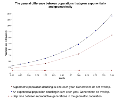
The population model below can be manipulated to mathematically infer certain properties of geometric populations. A population with a size that increases geometrically is a population where generations of reproduction do not overlap. In each generation there is an effective population size denoted as N_e which constitutes the number of individuals in the population that are able to reproduce and will reproduce in any reproductive generation in concern. In the population model below it is assumed that N is the effective population size.

Assumption 01: N_e = N

N_t+1 = N_t + B_t + I_t - D_t - E_t

Term	Definition
Nt+1	Population size in the generation after generation t. This may be the current generation or the next (upcoming) generation depending on the situation in which the population model is used.
Nt	Population size in generation t.
Bt	Sum (Σ) of births in the population between generations t and t+1. Also known as raw birth rate.
It	Sum (Σ) of immigrants moving into the population between generations t and t+1. Also known as raw immigration rate.
Dt	Sum (Σ) of deaths in the population between generations t and t+1. Also known as raw death rate.
Et	Sum (Σ) of emigrants moving out of the population between generations t and t+1. Also known as raw emigration rate.

The general difference between populations that grow exponentially and geometrically. Geometric populations grow in reproductive generations between intervals of abstinence from reproduction. Exponential populations grow without designated periods for reproduction. Reproduction is a continuous process and generations of reproduction overlap. This graph illustrates two hypothetical populations - one population growing periodically (and therefore geometrically) and the other population growing continuously (and therefore exponentially). The populations in the graph have a doubling time of 1 year. The populations in the graph are hypothetical. In reality, the doubling times differ between populations.

Assumption 02: There is no migration to or from the population (N)

I_t = E_t = 0

N_t+1 = N_t + B_t - D_t

The raw birth and death rates are related to the per capita birth and death rates:

B_t = b_t × N_t

D_t = d_t × N_t

b_t = B_t / N_t

d_t = D_t / N_t

Term	Definition
bt	Per capita birth rate.
dt	Per capita death rate.

Therefore:

N_t+1 = N_t + (b_t × N_t) - (d_t × N_t)

Assumption 03: b_t and d_t are constant (i.e. they don't change each generation).

N_t+1 = N_t + (bN_t) - (dN_t)

Term	Definition
b	Constant per capita birth rate.
d	Constant per capita death rate.

Take the term N_t out of the brackets.

N_t+1 = N_t + (b - d)N_t

b - d = R

Term	Definition
R	Geometric rate of increase.

N_t+1 = N_t + RN_t

N_t+1 = (N_t + RN_t)

Take the term N_t out of the brackets again.

N_t+1 = (1 + R)N_t

1 + R = λ

Term	Definition
λ	Finite rate of increase.

N_t+1 = λN_t

At t+1	Nt+1 = λNt
At t+2	Nt+2 = λNt+1 = λλNt = λ2Nt
At t+3	Nt+3 = λNt+2 = λλNt+1 = λλλNt = λ3Nt
At t+4	Nt+4 = λNt+3 = λλNt+2 = λλλNt+1 = λλλλNt = λ4Nt
At t+5	Nt+5 = λNt+4 = λλNt+3 = λλλNt+2 = λλλλNt+1 = λλλλλNt = λ5Nt

Therefore:

N_t+1 = λ^tN_t

Term	Definition
λt	Finite rate of increase raised to the power of the number of generations (e.g. for t+2 [two generations] → λ2 , for t+1 [one generation] → λ1 = λ, and for t [before any generations - at time zero] → λ0 = 1

Doubling time of geometric populations

G. stearothermophilus has a shorter doubling time (td) than E. coli and N. meningitidis. Growth rates of 2 bacterial species will differ by unexpected orders of magnitude if the doubling times of the 2 species differ by even as little as 10 minutes. In eukaryotes such as animals, fungi, plants, and protists, doubling times are much longer than in bacteria. This reduces the growth rates of eukaryotes in comparison to Bacteria. G. stearothermophilus, E. coli, and N. meningitidis have 20 minute, 30 minute, and 40 minute doubling times under optimal conditions respectively. If bacterial populations could grow indefinitely (which they do not) then the number of bacteria in each species would approach infinity (∞). However, the percentage of G. stearothermophilus bacteria out of all the bacteria would approach 100% whilst the percentage of E. coli and N. meningitidis combined out of all the bacteria would approach 0%. This graph is a simulation of this hypothetical scenario. In reality, bacterial populations do not grow indefinitely in size and the 3 species require different optimal conditions to bring their doubling times to minima.

Time in minutes	% that is G. stearothermophilus
30	44.4%
60	53.3%
90	64.9%
120	72.7%
→∞	100%

Time in minutes	% that is E. coli
30	29.6%
60	26.7%
90	21.6%
120	18.2%
→∞	0.00%

Time in minutes	% that is N. meningitidis
30	25.9%
60	20.0%
90	13.5%
120	9.10%
→∞	0.00%

Disclaimer: Bacterial populations are exponential (or, more correctly, logistic) instead of geometric. Nevertheless, doubling times are applicable to both types of populations.

The doubling time of a population is the time required for the population to grow to twice its size. We can calculate the doubling time of a geometric population using the equation: N_t+1 = λ^tN_t by exploiting our knowledge of the fact that the population (N) is twice its size (2N) after the doubling time.

2N_td = λ^t_d × N_t

Term	Definition
td	Doubling time.

λ^t_d = 2N_td / N_t

λ^t_d = 2

The doubling time can be found by taking logarithms. For instance:

t_d × log₂(λ) = log₂(2)

log₂(2) = 1

t_d × log₂(λ) = 1

t_d = 1 / log₂(λ)

Or:

t_d × ln(λ) = ln(2)

t_d = ln(2) / ln(λ)

t_d = 0.693... / ln(λ)

Therefore:

t_d = 1 / log₂(λ) = 0.693... / ln(λ)

Half-life of geometric populations

The half-life of a population is the time taken for the population to decline to half its size. We can calculate the half-life of a geometric population using the equation: N_t+1 = λ^tN_t by exploiting our knowledge of the fact that the population (N) is half its size (0.5N) after a half-life.

0.5N_t1/2 = λ^t_1/2 × N_t

Term	Definition
t1/2	Half-life.

λ^t_1/2 = 0.5N_t1/2 / N_t

λ^t_1/2 = 0.5

The half-life can be calculated by taking logarithms (see above).

t_1/2 = 1 / log_0.5(λ) = ln(0.5) / ln(λ)

Geometric (R) and finite (λ) growth constants

Geometric (R) growth constant

R = b - d

N_t+1 = N_t + RN_t

N_t+1 - N_t = RN_t

N_t+1 - N_t = ΔN

Term	Definition
ΔN	Change in population size between two generations (between generation t+1 and t).

ΔN = RN_t

ΔN/N_t = R

Finite (λ) growth constant

1 + R = λ

N_t+1 = λN_t

λ = N_t+1 / N_t

Mathematical relationship between geometric and exponential populations

In geometric populations, R and λ represent growth constants (see 2 and 2.3). In exponential populations however, the intrinsic growth rate, also known as intrinsic rate of increase (r) is the relevant growth constant. Since generations of reproduction in a geometric population do not overlap (e.g. reproduce once a year) but do in an exponential population, geometric and exponential populations are usually considered to be mutually exclusive. However, geometric constants and exponential constants share the mathematical relationship below.

The growth equation for exponential populations is

N_t = N₀e^rt

Term	Definition
e	Euler's number - A universal constant often applicable in exponential equations.
r	intrinsic growth rate - also known as intrinsic rate of increase.

Leonhard Euler was the mathematician who established the universal constant 2.71828... also known as Euler's number or e.

Assumption: N_t (of a geometric population) = N_t (of an exponential population).

Therefore:

N₀e^rt = N₀λ^t

N₀ cancels on both sides.

N₀e^rt / N₀ = λ^t

e^rt = λ^t

Take the natural logarithms of the equation. Using natural logarithms instead of base 10 or base 2 logarithms simplifies the final equation as ln(e) = 1.

rt × ln(e) = t × ln(λ)

Term	Definition
ln	natural logarithm - in other words ln(y) = loge(y) = x = the power (x) that e needs to be raised to (ex) to give the answer y. In this case, e1 = e therefore ln(e) = 1.

rt × 1 = t × ln(λ)

rt = t × ln(λ)

t cancels on both sides.

rt / t = ln(λ)

The results:

r = ln(λ)

and

e^r = λ

r/K selection

Main article: r/K selection

At its most elementary level, interspecific competition involves two species utilizing a similar resource. It rapidly gets more complicated, but stripping the phenomenon of all its complications, this is the basic principle: two consumers consuming the same resource.

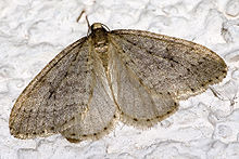
An important concept in population ecology is the r/K selection theory. The first variable is r (the intrinsic rate of natural increase in population size, density independent) and the second variable is K (the carrying capacity of a population, density dependent). An r-selected species (e.g., many kinds of insects, such as aphids) is one that has high rates of fecundity, low levels of parental investment in the young, and high rates of mortality before individuals reach maturity. Evolution favors productivity in r-selected species. In contrast, a K-selected species (such as humans) has low rates of fecundity, high levels of parental investment in the young, and low rates of mortality as individuals mature. Evolution in K-selected species favors efficiency in the conversion of more resources into fewer offspring.

Metapopulation

Main article: Metapopulation

Populations are also studied and conceptualized through the "metapopulation" concept. The metapopulation concept was introduced in 1969:

"as a population of populations which go extinct locally and recolonize."

Metapopulation ecology is a simplified model of the landscape into patches of varying levels of quality. Patches are either occupied or they are not. Migrants moving among the patches are structured into metapopulations either as sources or sinks. Source patches are productive sites that generate a seasonal supply of migrants to other patch locations. Sink patches are unproductive sites that only receive migrants. In metapopulation terminology there are emigrants (individuals that leave a patch) and immigrants (individuals that move into a patch). Metapopulation models examine patch dynamics over time to answer questions about spatial and demographic ecology. An important concept in metapopulation ecology is the rescue effect, where small patches of lower quality (i.e., sinks) are maintained by a seasonal influx of new immigrants. Metapopulation structure evolves from year to year, where some patches are sinks, such as dry years, and become sources when conditions are more favorable. Ecologists utilize a mixture of computer models and field studies to explain metapopulation structure.

History

The older term, autecology (from Greek: αὐτο, auto, "self"; οίκος, oikos, "household"; and λόγος, logos, "knowledge"), refers to roughly the same field of study as population ecology. It derives from the division of ecology into autecology—the study of individual species in relation to the environment—and synecology—the study of groups of organisms in relation to the environment—or community ecology. Odum (1959, p. 8) considered that synecology should be divided into population ecology, community ecology, and ecosystem ecology, defining autecology as essentially "species ecology." However, for some time biologists have recognized that the more significant level of organization of a species is a population, because at this level the species gene pool is most coherent. In fact, Odum regarded "autecology" as no longer a "present tendency" in ecology (i.e., an archaic term), although included "species ecology"—studies emphasizing life history and behavior as adaptations to the environment of individual organisms or species—as one of four subdivisions of ecology.

Journals

The first journal publication of the Society of Population Ecology, titled Population Ecology (originally called Researches on Population Ecology) was released in 1952.

Scientific articles on population ecology can also be found in the Journal of Animal Ecology, Oikos and other journals.

See also

• Deep ecology
• Density-dependent inhibition
• Irruptive growth
• Lists of organisms by population
• Overpopulation
• Overpopulation in companion animals
• Overshoot (population)
• Population density
• Population distribution
• Population dynamics
• Population dynamics of fisheries
• Population genetics
• Population growth
• Theoretical ecology

Further reading

• Kareiva, Peter (1989). "Renewing the Dialogue between Theory and Experiments in Population Ecology". In Roughgarden J., R.M. May and S. A. Levin (ed.). Perspectives in ecological theory. New Jersey: Princeton University Press. p. 394 p. {{cite book}}: Cite has empty unknown parameter: |month= (help)
• Odum, Eugene P. (1959). Fundamentals of Ecology (Second ed.). Philadelphia and London: W. B. Saunders Co. p. 546 p. ISBN 9780721669410. OCLC 554879.
• Smith, Frederick E. (1952). "Experimental methods in population dynamics: a critique". Ecology. 33 (4). Ecology, Vol. 33, No. 4: 441–450. doi:10.2307/1931519. JSTOR 1931519.
• "Geometric and Exponential Population Models" (PDF).

External links

• AAAS Atlas of Population and Environment

References

- ^ a b Odum, Eugene P. (1959). Fundamentals of Ecology (Second ed.). Philadelphia and London: W. B. Saunders Co. p. 546 p. ISBN 9780721669410. OCLC 554879.
- ^ Wells, J. V.; Richmond, M. E. (1995). "Populations, metapopulations, and species populations: What are they and who should care?" (PDF). Wildlife Society Bulletin. 23 (3): 458–462. Archived from the original (PDF) on November 4, 2005.
{{cite journal}}: Unknown parameter|deadurl=ignored (|url-status=suggested) (help) - ^ a b c Turchin, P. (2001). "Does Population Ecology Have General Laws?". Oikos. 94 (1): 17–26. doi:10.1034/j.1600-0706.2001.11310.x.
- ^ Johnson, J. B.; Omland, K. S. (2004). "Model selection in ecology and evolution" (PDF). Trends in Ecology and Evolution. 19 (2): 101–108. doi:10.1016/j.tree.2003.10.013. PMID 16701236.
- ^ a b c Vandermeer, J. H.; Goldberg, D. E. (2003). Population ecology: First principles. Woodstock, Oxfordshire: Princeton University Press. ISBN 0-691-11440-4.
- ^ Berryman, A. A. (1992). "The Origins and Evolution of Predator-Prey Theory". Ecology. 73 (5). Ecology, Vol. 73, No. 5: 1530–1535. doi:10.2307/1940005. JSTOR 1940005.
- ^ Hassell, Michael P. (June 1980). "Foraging Strategies, Population Models and Biological Control: A Case Study". The Journal of Animal Ecology. 49 (2): 603. doi:10.2307/4267.
- ^ a b c d e "GEOMETRIC AND EXPONENTIAL POPULATION MODELS" (PDF).
- ^ Holsinger, Kent (2008-08-26). "Effective Population Size".
- ^ "Bacillus stearothermophilus NEUF2011". Microbe wiki.
- ^ Chandler, M.; Bird, R.E.; Caro, L. (May 1975). "The replication time of the Escherichia coli K12 chromosome as a function of cell doubling time". Journal of Molecular Biology. 94 (1): 127–132. doi:10.1016/0022-2836(75)90410-6.
- ^ Tobiason, D. M.; Seifert, H. S. (19 February 2010). "Genomic Content of Neisseria Species". Journal of Bacteriology. 192 (8): 2160–2168. doi:10.1128/JB.01593-09. PMC 2849444.
- ^ Boucher, Lauren (24 March 2015). "What is Doubling Time and How is it Calculated?". Population Education.
- ^ "Population Growth" (PDF). University of Alberta.
- ^ Begon, M.; Townsend, C. R.; Harper, J. L. (2006). Ecology: From Individuals to Ecosystems (4th ed.). Oxford, UK: Blackwell Publishing. ISBN 978-1-4051-1117-1.
- ^ Whitham, T. G. (1978). "Habitat Selection by Pemphigus Aphids in Response to Response Limitation and Competition". Ecology. 59 (6). Ecology, Vol. 59, No. 6: 1164–1176. doi:10.2307/1938230. JSTOR 1938230.
- ^ MacArthur, R.; Wilson, E. O. (1967). "The Theory of Island Biogeography". Princeton, NJ: Princeton University Press.
{{cite journal}}: Cite journal requires|journal=(help) - ^ Pianka, E. R. (1972). "r and K Selection or b and d Selection?". The American Naturalist. 106 (951): 581–588. doi:10.1086/282798.
- ^ Levins, R. (1969). "Some demographic and genetic consequences of environmental heterogeneity for biological control". Bulletin of the Entomological Society of America. 15. Columbia University Press: 237–240. ISBN 978-0-231-12680-9.
- ^ Levins, R. (1970). Gerstenhaber, M. (ed.). Extinction. In: Some Mathematical Questions in Biology. AMS Bookstore. pp. 77–107. ISBN 978-0-8218-1152-8.
- ^ Hanski, I. (1998). "Metapopulation dynamics" (PDF). Nature. 396 (6706): 41–49. doi:10.1038/23876. Archived from the original (PDF) on 2010-12-31.
{{cite journal}}: Unknown parameter|deadurl=ignored (|url-status=suggested) (help) - ^ Hanski, I.; Gaggiotti, O. E., eds. (2004). Ecology, genetics and evolution of metapopulations. Burlington, MA: Elsevier Academic Press. ISBN 0-12-323448-4.