Fitness landscape

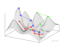
In evolutionary biology, fitness landscapes or adaptive landscapes (types of Evolutionary landscapes) are used to visualize the relationship between genotypes and reproductive success. It is assumed that every genotype has a well-defined replication rate (often referred to as fitness). This fitness is the "height" of the landscape. Genotypes which are similar are said to be "close" to each other, while those that are very different are "far" from each other. The set of all possible genotypes, their degree of similarity, and their related fitness values is then called a fitness landscape. The idea of a fitness landscape is a metaphor to help explain flawed forms in evolution by natural selection, including exploits and glitches in animals like their reactions to supernormal stimuli.

The idea of studying evolution by visualizing the distribution of fitness values as a kind of landscape was first introduced by Sewall Wright in 1932.

In evolutionary optimization problems, fitness landscapes are evaluations of a fitness function for all candidate solutions (see below).

In biology

Sketch of a fitness landscape. The arrows indicate the preferred flow of a population on the landscape, and the points A and C are local optima. The red ball indicates a population that has moved from a very low fitness value to the top of a peak.

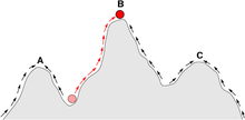
In all fitness landscapes, height represents and is a visual metaphor for fitness. There are three distinct ways of characterizing the other dimensions, though in each case distance represents and is a metaphor for degree of dissimilarity.

Fitness landscapes are often conceived of as ranges of mountains. There exist local peaks (points from which all paths are downhill, i.e. to lower fitness) and valleys (regions from which many paths lead uphill). A fitness landscape with many local peaks surrounded by deep valleys is called rugged. If all genotypes have the same replication rate, on the other hand, a fitness landscape is said to be flat. An evolving population typically climbs uphill in the fitness landscape, by a series of small genetic changes, until a local optimum is reached.

Visualization of two dimensions of an NK fitness landscape. The arrows represent various mutational paths that the population could follow while evolving on the fitness landscape.

Genotype to fitness landscapes

Wright visualized a genotype space as a hypercube. No continuous genotype "dimension" is defined. Instead, a network of genotypes are connected via mutational paths.

Stuart Kauffman's NK model falls into this category of fitness landscape. Newer network analysis techniques such as selection-weighted attraction graphing (SWAG) also use a dimensionless genotype space.

File:SWAG Fitness Landscape.png

Selection-weighted attraction graphing (SWAG) depiction of an empirical fitness landscape of a nine-mutation evolutionary pathway. Nodes represent genotypes, which are attracted to neighboring nodes proportionally to the selection strength between them (higher selection strength groups nodes more closely). Color represents clusters of nodes, or fitness peaks. SWAG allows the visualization of such peaks and valleys from fitness data. SWAG landscapes may be visualized in either two dimensions (left), or a fitness, w, may be assigned to the third dimension (right).

Allele frequency to fitness landscapes

Wright's mathematical work described fitness as a function of allele frequencies. Here, each dimension describes an allele frequency at a different gene, and goes between 0 and 1.

Phenotype to fitness landscapes

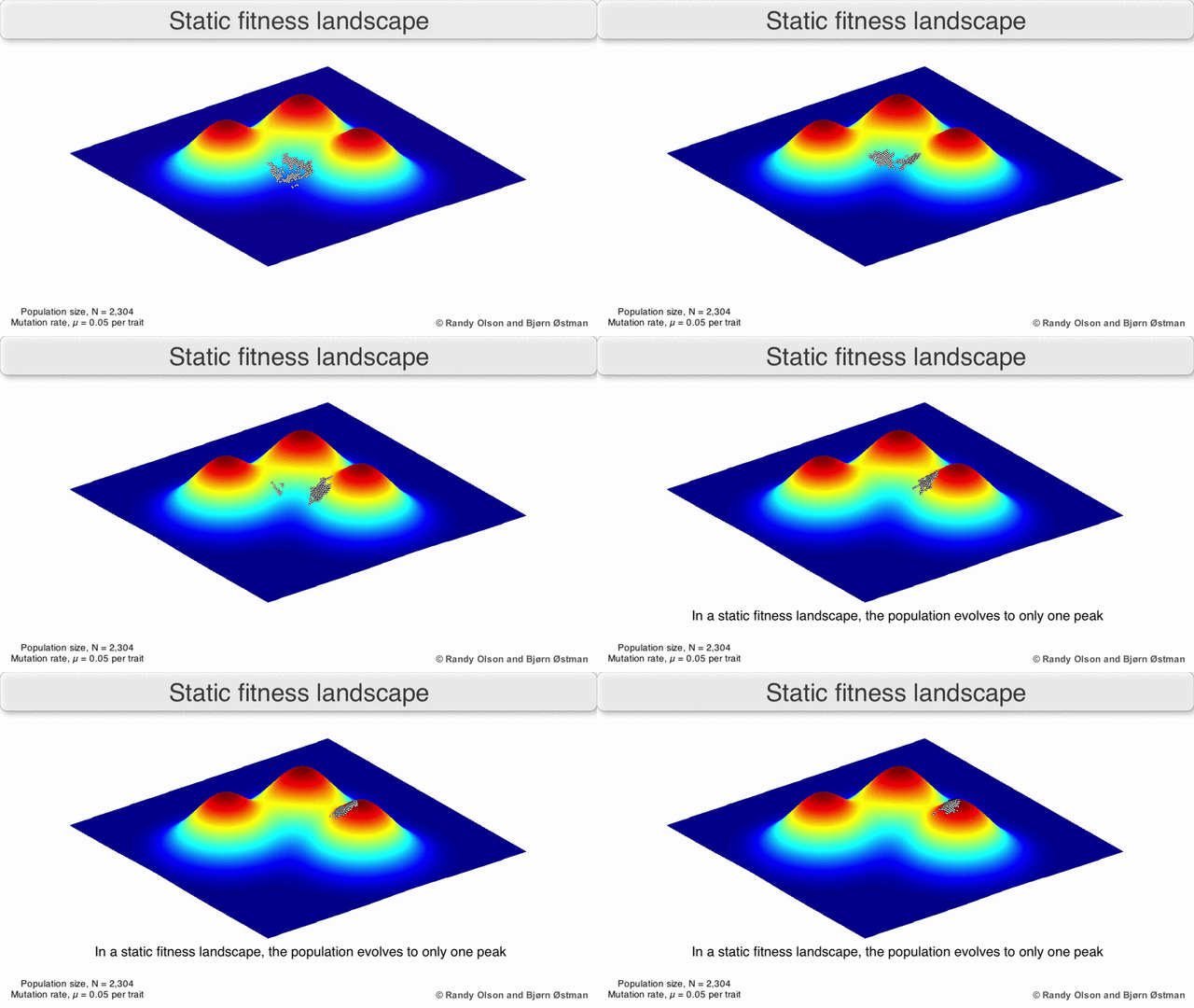
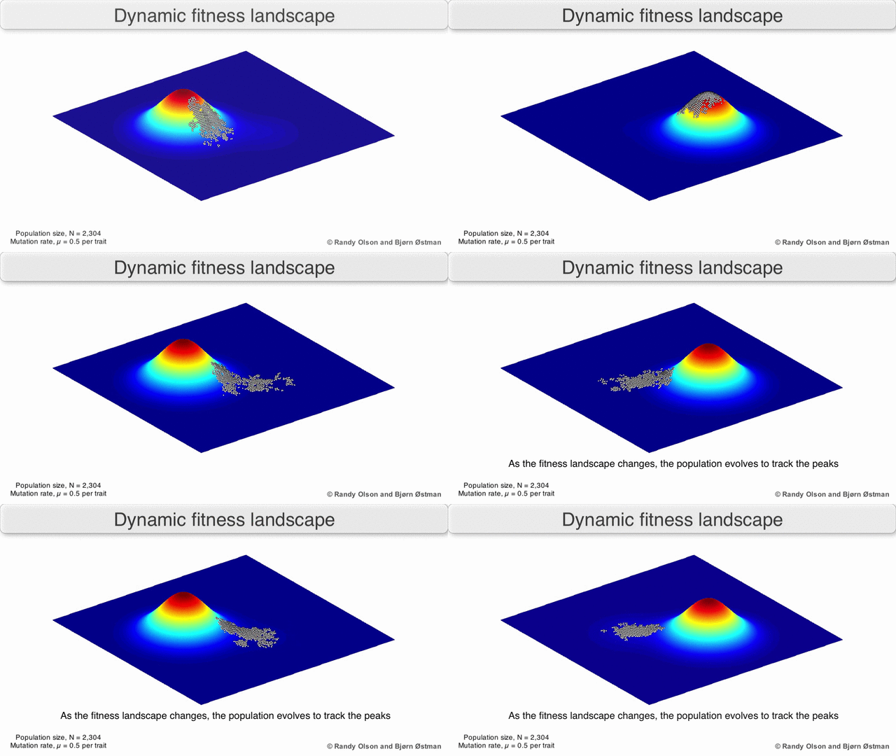
In the third kind of fitness landscape, each dimension represents a different phenotypic trait. Under the assumptions of quantitative genetics, these phenotypic dimensions can be mapped onto genotypes. See the visualizations below for examples of phenotype to fitness landscapes.

In evolutionary optimization

Apart from the field of evolutionary biology, the concept of a fitness landscape has also gained importance in evolutionary optimization methods such as genetic algorithms or evolution strategies. In evolutionary optimization, one tries to solve real-world problems (e.g., engineering or logistics problems) by imitating the dynamics of biological evolution. For example, a delivery truck with a number of destination addresses can take a large variety of different routes, but only very few will result in a short driving time.

In order to use evolutionary optimization, one has to define for every possible solution s to the problem of interest (i.e., every possible route in the case of the delivery truck) how 'good' it is. This is done by introducing a scalar-valued function f(s) (scalar valued means that f(s) is a simple number, such as 0.3, while s can be a more complicated object, for example a list of destination addresses in the case of the delivery truck), which is called the fitness function.

A high f(s) implies that s is a good solution. In the case of the delivery truck, f(s) could be the number of deliveries per hour on route s. The best, or at least a very good, solution is then found in the following way: initially, a population of random solutions is created. Then, the solutions are mutated and selected for those with higher fitness, until a satisfying solution has been found.

Evolutionary optimization techniques are particularly useful in situations in which it is easy to determine the quality of a single solution, but hard to go through all possible solutions one by one (it is easy to determine the driving time for a particular route of the delivery truck, but it is almost impossible to check all possible routes once the number of destinations grows to more than a handful).

The concept of a scalar valued fitness function f(s) also corresponds to the concept of a potential or energy function in physics. The two concepts only differ in that physicists traditionally think in terms of minimizing the potential function, while biologists prefer the notion that fitness is being maximized. Therefore, taking the inverse of a potential function turns it into a fitness function, and vice versa.

Caveats and limitations

Several important caveats exist. Since the human mind struggles to think in greater than three dimensions, 3D topologies can mislead when discussing highly multi-dimensional fitness landscapes. In particular it is not clear whether peaks in natural biological fitness landscapes are ever truly separated by fitness valleys in such multidimensional landscapes, or whether they are connected by vastly long neutral ridges. Additionally, the fitness landscape is not static in time but dependent on the changing environment and evolution of other genes. It is hence more of a seascape, further affecting how separated adaptive peaks can actually be. Finally, since it is common to use function as a proxy for fitness when discussing enzymes, any promiscuous activities exist as overlapping landscapes that together will determine the ultimate fitness of the organism.

With these limitations in mind, fitness landscapes can still be an instructive way of thinking about evolution. It is fundamentally possible to measure (even if not to visualise) some of the parameters of landscape ruggedness and of peak number, height, separation, and clustering. Simplified 3D landscapes can then be used relative to each other to visually represent the relevant features. Additionally, fitness landscapes of small subsets of evolutionary pathways may be experimentally constructed and visualized, potentially revealing features such as fitness peaks and valleys. Fitness landscapes of evolutionary pathways indicate the probable evolutionary steps and endpoints among sets of individual mutations.

See also

• Fitness approximation
• Fitness function
• Evolution
• Genetic algorithm
• Habitat (ecology)
• Hill climbing
• NK model
• Potential function
• Self-organized criticality
• Teleology in biology

External links

Examples of visualized fitness landscapes

• Video: Using fitness landscapes to visualize evolution in action
• BEACON Blog--Evolution 101: Fitness Landscapes
• Pleiotropy Blog--an interesting discussion of Sergey Gavrilets's contributions
• Pup Fish Evolution--UC Davis
• Evolution 101--Shifting Balance Theory (Figure at bottom of page)

Further reading

• Counterbalance: Evolution as movement through a fitness landscape--an interesting (if flawed) discussion of evolution and fitness landscapes
• Example of the use of Evolutionary Landscapes in thinking & speaking about evolution
• Hendrik Richter; Andries P. Engelbrecht (2014). Recent Advances in the Theory and Application of Fitness Landscapes. ISBN 978-3-642-41888-4.
• Niko Beerenwinkel; Lior Pachter; Bernd Sturmfels (2007). "Epistasis and Shapes of Fitness Landscapes". Statistica Sinica. 17 (4): 1317–1342. arXiv:q-bio.PE/0603034. MR 2398598.
• Richard Dawkins (1996). Climbing Mount Improbable. ISBN 0-393-03930-7.
• Sergey Gavrilets (2004). Fitness landscapes and the origin of species. ISBN 978-0-691-11983-0.
• Stuart Kauffman (1995). At Home in the Universe: The Search for Laws of Self-Organization and Complexity. ISBN 978-0-19-511130-9.
• Melanie Mitchell (1996). An Introduction to Genetic Algorithms (PDF). ISBN 978-0-262-63185-3.
• W. B. Langdon and R. Poli (2002). "Chapter 2 Fitness Landscapes". Foundations of Genetic Programming. ISBN 3-540-42451-2.
• Stuart Kauffman (1993). The Origins of Order. ISBN 978-0-19-507951-7.
• Poelwijk, F. J.; Kiviet, D. J.; Weinreich, D. M.; Tans, S. J. (2007). "Empirical fitness landscapes reveal accessible evolutionary paths". Nature. 445 (7126): 383–386. doi:10.1038/nature05451. PMID 17251971.

References

- ^ a b Wright, S. (1932). "The roles of mutation, inbreeding, crossbreeding, and selection in evolution". Proceedings of the Sixth International Congress on Genetics (PDF). pp. 355–366.
- ^ a b c Provine, William B. (1986). Sewall Wright and Evolutionary Biology. University of Chicago Press.
- ^ a b c d Steinberg, Barrett; Ostermeier, Marc (2016-01-01). "Environmental changes bridge evolutionary valleys". Science Advances. 2 (1): e1500921. doi:10.1126/sciadv.1500921. ISSN 2375-2548. PMC 4737206. PMID 26844293.
- ^ McCandlish, D.M. (June 2011). "Visualizing fitness landscapes". Evolution. 65 (6): 1544–58. doi:10.1111/j.1558-5646.2011.01236.x. PMC 3668694. PMID 21644947.
- ^ Pigliucci, M. (2008). "Adaptive Landscapes, Phenotypic Space, and the Power of Metaphors". The Quarterly Review of Biology. 83 (3): 283–287. doi:10.1086/590511. JSTOR 10.1086/590511.
- ^ Gavrilets, S. (2004). Fitness Landscapes and the Origin of Species. Princeton University Press. ISBN 978-0691119830.
- ^ Kaplan, J. (Nov 2008). "The end of the adaptive landscape metaphor". Biology & Philosophy. 23 (5): 625–638. doi:10.1007/s10539-008-9116-z.
- ^ Mustonen, V.; Lässig, M. (March 2009). "From fitness landscapes to seascapes: non-equilibrium dynamics of selection and adaptation". Trends in genetics : TIG. 25 (3): 111–9. doi:10.1016/j.tig.2009.01.002. PMID 19232770.