Skewness

Example of experimental data with non-zero skewness (gravitropic response of wheat coleoptiles, 1,790)

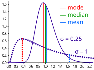
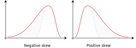
In probability theory and statistics, skewness is a measure of the asymmetry of the probability distribution of a real-valued random variable. The skewness value can be positive or negative, or even undefined. Qualitatively, a negative skew indicates that the tail on the left side of the probability density function is longer than the right side and the bulk of the values (possibly including the median) lie to the right of the mean. A positive skew indicates that the tail on the right side is longer than the left side and the bulk of the values lie to the left of the mean. A zero value indicates that the values are relatively evenly distributed on both sides of the mean, typically but not necessarily implying a symmetric distribution.

Introduction

Consider the distribution on the figure. The bars on the right side of the distribution taper differently than the bars on the left side. These tapering sides are called tails, and they provide a visual means for determining which of the two kinds of skewness a distribution has:

1. negative skew: The left tail is longer; the mass of the distribution is concentrated on the right of the figure. It has relatively few low values. The distribution is said to be left-skewed or "skewed to the left". Example (observations): 1,1000,1001,1002,1003
2. positive skew: The right tail is longer; the mass of the distribution is concentrated on the left of the figure. It has relatively few high values. The distribution is said to be right-skewed or "skewed to the right". Example (observations): 1,2,3,4,100.

If the distribution is symmetric then the mean = median and there is zero skewness. (If, in addition, the distribution is unimodal, then the mean = median = mode.) This is the case of a coin toss or the series 1,2,3,4,... Note, however, that the converse is not true in general, i.e. zero skewness does not imply that the mean = median.

"Many textbooks," a 2005 article points out, "teach a rule of thumb stating that the mean is right of the median under right skew, and left of the median under left skew. [But] this rule fails with surprising frequency. It can fail in multimodal distributions, or in distributions where one tail is long but the other is heavy. Most commonly, though, the rule fails in discrete distributions where the areas to the left and right of the median are not equal. Such distributions not only contradict the textbook relationship between mean, median, and skew, they also contradict the textbook interpretation of the median."

Definition

The skewness of a random variable X is the third standardized moment, denoted γ₁ and defined as

$\gamma _{1}=\operatorname {E} {\Big [}{\big (}{\tfrac {X-\mu }{\sigma }}{\big )}^{\!3}\,{\Big ]}={\frac {\mu _{3}}{\sigma ^{3}}}={\frac {\operatorname {E} {\big [}(X-\mu )^{3}{\big ]}}{\ \ \ (\operatorname {E} {\big [}(X-\mu )^{2}{\big ]})^{3/2}}}={\frac {\kappa _{3}}{\kappa _{2}^{3/2}}}\ ,$

where μ₃ is the third moment about the mean μ, σ is the standard deviation, and E is the expectation operator. The last equality expresses skewness in terms of the ratio of the third cumulant κ₃ and the 1.5th power of the second cumulant κ₂. This is analogous to the definition of kurtosis as the fourth cumulant normalized by the square of the second cumulant.

The skewness is also sometimes denoted Skew[X].

The formula expressing skewness in terms of the non-central moment E[X³] can be expressed by expanding the previous formula,

$\gamma _{1}=\operatorname {E} {\bigg [}{\Big (}{\frac {X-\mu }{\sigma }}{\Big )}^{\!3}\,{\bigg ]}={\frac {\operatorname {E} [X^{3}]-3\mu \operatorname {E} [X^{2}]+3\mu ^{3}-\mu ^{3}}{\sigma ^{3}}}={\frac {\operatorname {E} [X^{3}]-3\mu \sigma ^{2}-\mu ^{3}}{\sigma ^{3}}}\ .$

Sample skewness

For a sample of n values the sample skewness is

$g_{1}={\frac {m_{3}}{m_{2}^{3/2}}}={\frac {{\tfrac {1}{n}}\sum _{i=1}^{n}(x_{i}-{\overline {x}})^{3}}{\left({\tfrac {1}{n}}\sum _{i=1}^{n}(x_{i}-{\overline {x}})^{2}\right)^{3/2}}}\ ,$

where $\scriptstyle {\overline {x}}$ is the sample mean, m₃ is the sample third central moment, and m₂ is the sample variance.

Given samples from a population, the equation for the sample skewness $g_{1}$ above is a biased estimator of the population skewness. (Note that for a discrete distribution the sample skewness may be undefined (0/0), so its expected value will be undefined.) The usual estimator of population skewness is

$G_{1}={\frac {k_{3}}{k_{2}^{3/2}}}={\frac {\sqrt {n\,(n-1)}}{n-2}}\;g_{1},$

where $k_{3}$ is the unique symmetric unbiased estimator of the third cumulant and $k_{2}$ is the symmetric unbiased estimator of the second cumulant. Unfortunately $G_{1}$ is, nevertheless, generally biased (although it obviously has the correct expected value of zero for a symmetric distribution). Its expected value can even have the opposite sign from the true skewness. For instance a mixed distribution consisting of very thin Gaussians centred at −99, 0.5, and 2 with weights 0.01, 0.66, and 0.33 has a skewness of about −9.77, but in a sample of 3, $G_{1}$ has an expected value of about 0.32, since usually all three samples are in the positive-valued part of the distribution, which is skewed the other way.

Properties

Skewness can be infinite, as when

$\Pr \left[X>x\right]=x^{-3}{\mbox{ for }}x>1,\ \Pr[X<1]=0$

or undefined, as when

$\Pr[X<x]=(1-x)^{-3}/2{\mbox{ for negative }}x{\mbox{ and }}\Pr[X>x]=(1+x)^{-3}/2{\mbox{ for positive }}x.$

In this latter example, the third cumulant is undefined. One can also have distributions such as

$\Pr \left[X>x\right]=x^{-2}{\mbox{ for }}x>1,\ \Pr[X<1]=0$

where both the second and third cumulants are infinite, so the skewness is again undefined.

If Y is the sum of n independent and identically distributed random variables, all with the distribution of X, then the third cumulant of Y is n times that of X and the second cumulant of Y is n times that of X, so ${\mbox{Skew}}[Y]={\mbox{Skew}}[X]/{\sqrt {n}}$. This shows that the skewness of the sum is smaller, as it approaches a Gaussian distribution in accordance with the central limit theorem.

Applications

Skewness has benefits in many areas. Many models assume normal distribution; i.e., data are symmetric about the mean. The normal distribution has a skewness of zero. But in reality, data points may not be perfectly symmetric. So, an understanding of the skewness of the dataset indicates whether deviations from the mean are going to be positive or negative.

D'Agostino's K-squared test is a goodness-of-fit normality test based on sample skewness and sample kurtosis.

Other measures of skewness

Pearson's skewness coefficients

Comparison of mean, median and mode of two log-normal distributions with different skewness.

Karl Pearson suggested simpler calculations as a measure of skewness: the Pearson mode or first skewness coefficient, defined by

• (mean − mode) / standard deviation,

as well as Pearson's median or second skewness coefficient, defined by

• 3 (mean − median) / standard deviation.

Starting from a standard cumulant expansion around a Normal distribution, one can actually show that skewness = 6 (mean − median) / standard deviation ( 1 + kurtosis / 8) + O(skewness²). One should keep in mind that above given equalities often don't hold even approximately and these empirical formulas are abandoned nowadays. There is no guarantee that these will be the same sign as each other or as the ordinary definition of skewness.

Quantile based measures

A skewness function

$\gamma (u)={\frac {F^{-1}(u)+F^{-1}(1-u)-2F^{-1}(1/2)}{F^{-1}(u)-F^{-1}(1-u)}}$

can be defined, where F is the cumulative distribution function. This leads to a corresponding overall measure of skewness defined as the supremum of this over the range 1/2≤u<1, while another measure can be obtained by integrating the numerator and denominator of this expression. Galton's measure of skewness is γ(u) evaluated at u=3/4, while other names for this same quantity are "Bowley Skewness", "Yule-Kendall index" and "quartile skewness". The function γ(u) satifies -1≤γ(u)≤1, and is well-defined without requiring the existence of any moments of the distribution.

L-moments

Use of L-moments in place of moments provides a measure of skewness known as the L-skewness.

Cyhelský’s skewness coefficient

A simple skewness coefficient derived from the sample mean and individual observations:

a = ( number of observations below the mean - number of observations above the mean ) / total number of observations

The skewness coefficient a approaches to normal distribution. If data set has at least 45 values then a is nearly normal. Distribution of a if data are taken from normal or uniform distribution is the same. Behavior of a in other distributions is currently unknown. Although this measure is very easy to understand, analytic approach is difficult.

Distance skewness

A value of skewness equal to zero does not imply that the probability distribution is symmetric. Thus there is a need for another measure of asymmetry which has this property: such a measure was introduced in 2000. It is called distance skewness and denoted by dSkew. If X is a random variable which takes values in the d-dimensional Euclidean space, X has finite expectation, X’ is an independent identically distributed copy of X and || . || denotes the norm in the Euclidean space then a simple measure of asymmetry is

dSkew (X) := 1 - E||X-X’|| / E||X + X’|| if X is not 0 with probability one,

and dSkew (X):= 1 for X = 0 (with probability 1). Distance skewness is always between 0 and 1, equals 0 if and only if X is diagonally symmetric (X and -X has the same probability distribution) and equals 1 if and only if X is a nonzero constant with probability one. Thus there is a simple consistent statistical test of diagonal symmetry based on the sample distance skewness:

dSkew_n(X):= 1- ∑_i,j ||x_i – x_j|| / ∑_i,j||x_i + x_j||.

See also

• Skewness risk
• Kurtosis risk
• Shape parameters
• Skew normal distribution
• D'Agostino's K-squared test

References

• Groeneveld, RA; Meeden, G. (1984). "Measuring Skewness and Kurtosis". The Statistician. 33 (4): 391–399. doi:10.2307/2987742.
• Johnson, NL, Kotz, S, Balakrishnan N (1994) Continuous Univariate Distributions, Vol 1, 2nd Edition Wiley ISBN0-471-58495-9
• MacGillivray, HL (1992). "Shape properties of the g- and h- and Johnson families". Comm. Statistics - Theory and Methods. 21: 1244–1250.

External links

• An Asymmetry Coefficient for Multivariate Distributions by Michel Petitjean
• On More Robust Estimation of Skewness and Kurtosis Comparison of skew estimators by Kim and White.
• Closed-skew Distributions - Simulation, Inversion and Parameter Estimation