Maximum likelihood estimation

In statistics, maximum-likelihood estimation (MLE) is a method of estimating the parameters of a statistical model. When applied to a data set and given a statistical model, maximum-likelihood estimation provides estimates for the model's parameters.

The method of maximum likelihood corresponds to many well-known estimation methods in statistics. For example, one may be interested in the heights of adult female giraffes, but be unable to measure the height of every single giraffe in a population due to cost or time constraints. Assuming that the heights are normally (Gaussian) distributed with some unknown mean and variance, the mean and variance can be estimated with MLE while only knowing the heights of some sample of the overall population. MLE would accomplish this by taking the mean and variance as parameters and finding particular parametric values that make the observed results the most probable (given the model).

In general, for a fixed set of data and underlying statistical model, the method of maximum likelihood selects values of the model parameters that produce a distribution that gives the observed data the greatest probability (i.e., parameters that maximize the likelihood function). Maximum-likelihood estimation gives a unified approach to estimation, which is well-defined in the case of the normal distribution and many other problems. However, in some complicated problems, difficulties do occur: in such problems, maximum-likelihood estimators are unsuitable or do not exist.

Principles

Suppose there is a sample x₁, x₂, …, x_n of n independent and identically distributed observations, coming from a distribution with an unknown pdf ƒ₀(·). It is however surmised that the function ƒ₀ belongs to a certain family of distributions { ƒ(·|θ), θ ∈ Θ }, called the parametric model, so that ƒ₀ = ƒ(·|θ₀). The value θ₀ is unknown and is referred to as the "true value" of the parameter. It is desirable to find an estimator $\scriptstyle {\hat {\theta }}$ which would be as close to the true value θ₀ as possible. Both the observed variables x_i and the parameter θ can be vectors.

To use the method of maximum likelihood, one first specifies the joint density function for all observations. For an iid sample, this joint density function is

$f(x_{1},x_{2},\ldots ,x_{n}\;|\;\theta )=f(x_{1}|\theta )\cdot f(x_{2}|\theta )\cdots f(x_{n}|\theta ).$

Now we look at this function from a different perspective by considering the observed values x₁, x₂, ..., x_n to be fixed "parameters" of this function, whereas θ will be the function's variable and allowed to vary freely; this function will be called the likelihood:

${\mathcal {L}}(\theta \,|\,x_{1},\ldots ,x_{n})=f(x_{1},x_{2},\ldots ,x_{n}\;|\;\theta )=\prod _{i=1}^{n}f(x_{i}|\theta ).$

In practice it is often more convenient to work with the logarithm of the likelihood function, called the log-likelihood:

$\ln {\mathcal {L}}(\theta \,|\,x_{1},\ldots ,x_{n})=\sum _{i=1}^{n}\ln f(x_{i}|\theta ),$

or the average log-likelihood':

${\hat {\ell }}={\frac {1}{n}}\ln {\mathcal {L}}.$

The hat over $\scriptstyle \ell$ indicates that it is akin to some estimator. Indeed, $\scriptstyle {\hat {\ell }}$ estimates the expected log-likelihood of a single observation in the model.

The method of maximum likelihood estimates θ₀ by finding a value of θ that maximizes $\scriptstyle {\hat {\ell }}(\theta |x)$. This method of estimation defines a maximum-likelihood estimator (MLE) of θ₀

$\{{\hat {\theta }}_{\mathrm {mle} }\}\subseteq \{{\underset {\theta \in \Theta }{\operatorname {arg\,max} }}\ {\hat {\ell }}(\theta \,|\,x_{1},\ldots ,x_{n})\}.$

if any maximum exists. An MLE estimate is the same regardless of whether we maximize the likelihood or the log-likelihood function, since log is a monotone transformation.

For many models, a maximum likelihood estimator can be found as an explicit function of the observed data x₁, …, x_n. For many other models, however, no closed-form solution to the maximization problem is known or available, and an MLE has to be found numerically using optimization methods. For some problems, there may be multiple estimates that maximize the likelihood. For other problems, no maximum likelihood estimate exists (meaning that the log-likelihood function increases without attaining the supremum value).

In the exposition above, it is assumed that the data are independent and identically distributed. The method can be applied however to a broader setting, as long as it is possible to write the joint density function ƒ(x₁,…,x_n | θ), and its parameter θ has a finite dimension which does not depend on the sample size n. In a simpler extension, an allowance can be made for data heterogeneity, so that the joint density is equal to ƒ₁(x₁|θ) · ƒ₂(x₂|θ) · … · ƒ_n(x_n|θ). In the more complicated case of time series models, the independence assumption may have to be dropped as well.

A maximum likelihood estimator coincides with the most probable Bayesian estimator given a uniform prior distribution on the parameters.

Properties

A maximum-likelihood estimator is an extremum estimator obtained by maximizing, as a function of θ, the objective function

${\hat {\ell }}(\theta |x)={\frac {1}{n}}\sum _{i=1}^{n}\ln f(x_{i}|\theta ),$

this being the sample analogue of the expected log-likelihood $\scriptstyle \ell (\theta )=\operatorname {E} [\,\ln f(x_{i}|\theta )\,]$, where this expectation is taken with respect to the true density f(·|θ₀).

Maximum-likelihood estimators have no optimum properties for finite samples, in the sense that (when evaluated on finite samples) other estimators have greater concentration around the true parameter-value. However, like other estimation methods, maximum-likelihood estimation possesses a number of attractive limiting properties: As the sample-size increases to infinity, sequences of maximum-likelihood estimators have these properties:

• Consistency: a subsequence of the sequence of MLEs converges in probability to the value being estimated.
• Asymptotic normality: as the sample size increases, the distribution of the MLE tends to the Gaussian distribution with mean $\theta$ and covariance matrix equal to the inverse of the Fisher information matrix.
• Efficiency, i.e., it achieves the Cramér–Rao lower bound when the sample size tends to infinity. This means that no asymptotically unbiased estimator has lower asymptotic mean squared error than the MLE (or other estimators attaining this bound).
• Second-order efficiency after correction for bias.

Consistency

Under the conditions outlined below, the maximum likelihood estimator is consistent. The consistency means that having a sufficiently large number of observations n, it is possible to find the value of θ₀ with arbitrary precision. In mathematical terms this means that as n goes to infinity the estimator $\scriptstyle {\hat {\theta }}$ converges in probability to its true value:

${\hat {\theta }}_{\mathrm {mle} }\ {\xrightarrow {p}}\ \theta _{0}.$

Under slightly stronger conditions, the estimator converges almost surely (or strongly) to:

${\hat {\theta }}_{\mathrm {mle} }\ {\xrightarrow {\text{a.s.}}}\ \theta _{0}.$

To establish consistency, the following conditions are sufficient:

1. Identification of the model:

   $\theta \neq \theta _{0}\quad \Leftrightarrow \quad f(\cdot |\theta )\neq f(\cdot |\theta _{0}).$

   In other words, different parameter values θ correspond to different distributions within the model. If this condition did not hold, there would be some value θ₁ such that θ₀ and θ₁ generate an identical distribution of the observable data. Then we wouldn't be able to distinguish between these two parameters even with an infinite amount of data — these parameters would have been observationally equivalent.
   The identification condition is absolutely necessary for the ML estimator to be consistent. When this condition holds, the limiting likelihood function ℓ(θ|·) has unique global maximum at θ₀.
2. Compactness: the parameter space Θ of the model is compact.

   

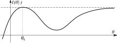
   The identification condition establishes that the log-likelihood has a unique global maximum. Compactness implies that the likelihood cannot approach the maximum value arbitrarily close at some other point (as demonstrated for example in the picture on the right).

   Compactness is only a sufficient condition and not a necessary condition. Compactness can be replaced by some other conditions, such as:

   • both concavity of the log-likelihood function and compactness of some (nonempty) upper level sets of the log-likelihood function, or
   • existence of a compact neighborhood N of θ₀ such that outside of N the log-likelihood function is less than the maximum by at least some ε > 0.
3. Continuity: the function ln f(x|θ) is continuous in θ for almost all values of x:

   $\Pr \!{\big [}\;\ln f(x\,|\,\theta )\;\in \;\mathbb {C} ^{0}(\Theta )\;{\big ]}=1.$

   The continuity here can be replaced with a slightly weaker condition of upper semi-continuity.
4. Dominance: there exists an integrable function D(x) such that

   ${\big |}\ln f(x\,|\,\theta ){\big |}<D(x)\quad {\text{for all}}\ \theta \in \Theta .$

   By the uniform law of large numbers, the dominance condition together with continuity establish the uniform convergence in probability of the log-likelihood:

   $\sup _{\theta \in \Theta }{\big |}\,{\hat {\ell }}(\theta |x)-\ell (\theta )\,{\big |}\ {\xrightarrow {p}}\ 0.$

The dominance condition can be employed in the case of i.i.d. observations. In the non-i.i.d. case the uniform convergence in probability can be checked by showing that the sequence $\scriptstyle {\hat {\ell }}(\theta |x)$ is stochastically equicontinuous.

If one wants to demonstrate that the ML estimator $\scriptstyle {\hat {\theta }}$ converges to θ₀ almost surely, then a stronger condition of uniform convergence almost surely has to be imposed:

$\sup _{\theta \in \Theta }{\big \|}\;{\hat {\ell }}(x|\theta )-\ell (\theta )\;{\big \|}\ {\xrightarrow {\text{a.s.}}}\ 0.$

Asymptotic normality

Maximum-likelihood estimators can lack asymptotic normality and can be inconsistent if there is a failure of one (or more) of the below regularity conditions:

Estimate on boundary. Sometimes the maximum likelihood estimate lies on the boundary of the set of possible parameters, or (if the boundary is not, strictly speaking, allowed) the likelihood gets larger and larger as the parameter approaches the boundary. Standard asymptotic theory needs the assumption that the true parameter value lies away from the boundary. If we have enough data, the maximum likelihood estimate will keep away from the boundary too. But with smaller samples, the estimate can lie on the boundary. In such cases, the asymptotic theory clearly does not give a practically useful approximation. Examples here would be variance-component models, where each component of variance, σ², must satisfy the constraint σ² ≥0.

Data boundary parameter-dependent. For the theory to apply in a simple way, the set of data values which has positive probability (or positive probability density) should not depend on the unknown parameter. A simple example where such parameter-dependence does hold is the case of estimating θ from a set of independent identically distributed when the common distribution is uniform on the range (0,θ). For estimation purposes the relevant range of θ is such that θ cannot be less than the largest observation. Because the interval (0,θ) is not compact, there exists no maximum for the likelihood function: For any estimate of theta, there exists a greater estimate that also has greater likelihood. In contrast, the interval [0,θ] includes the end-point θ and is compact, in which case the maximum-likelihood estimator exists. However, in this case, the maximum-likelihood estimator is biased. Asymptotically, this maximum-likelihood estimator is not normally distributed.

Nuisance parameters. For maximum likelihood estimations, a model may have a number of nuisance parameters. For the asymptotic behaviour outlined to hold, the number of nuisance parameters should not increase with the number of observations (the sample size). A well-known example of this case is where observations occur as pairs, where the observations in each pair have a different (unknown) mean but otherwise the observations are independent and Normally distributed with a common variance. Here for 2N observations, there are N+1 parameters. It is well known that the maximum likelihood estimate for the variance does not converge to the true value of the variance.

Increasing information. For the asymptotics to hold in cases where the assumption of independent identically distributed observations does not hold, a basic requirement is that the amount of information in the data increases indefinitely as the sample size increases. Such a requirement may not be met if either there is too much dependence in the data (for example, if new observations are essentially identical to existing observations), or if new independent observations are subject to an increasing observation error.

Some regularity conditions which ensure this behavior are:

1. The first and second derivatives of the log-likelihood function must be defined.
2. The Fisher information matrix must not be zero, and must be continuous as a function of the parameter.
3. The maximum likelihood estimator is consistent.

Suppose that conditions for consistency of maximum likelihood estimator are satisfied, and

1. θ₀ ∈ interior(Θ);
2. f(x|θ) > 0 and is twice continuously differentiable in θ in some neighborhood N of θ₀;
3. ∫ sup_θ∈N||∇_θf(x|θ)||dx < ∞, and ∫ sup_θ∈N||∇_θθf(x|θ)||dx < ∞;
4. I = E[∇_θlnf(x|θ₀) ∇_θlnf(x|θ₀)′] exists and is nonsingular;
5. E[ sup_θ∈N||∇_θθlnf(x|θ)||] < ∞.

Then the maximum likelihood estimator has asymptotically normal distribution:

${\sqrt {n}}{\big (}{\hat {\theta }}_{\mathrm {mle} }-\theta _{0}{\big )}\ {\xrightarrow {d}}\ {\mathcal {N}}(0,\,I^{-1}).$

Proof, skipping the technicalities:

Since the log-likelihood function is differentiable, and θ₀ lies in the interior of the parameter set, in the maximum the first-order condition will be satisfied:

$\nabla _{\!\theta }\,{\hat {\ell }}({\hat {\theta }}|x)={\frac {1}{n}}\sum _{i=1}^{n}\nabla _{\!\theta }\ln f(x_{i}|{\hat {\theta }})=0.$

When the log-likelihood is twice differentiable, this expression can be expanded into a Taylor series around the point θ = θ₀:

$0={\frac {1}{n}}\sum _{i=1}^{n}\nabla _{\!\theta }\ln f(x_{i}|\theta _{0})+{\Bigg [}\,{\frac {1}{n}}\sum _{i=1}^{n}\nabla _{\!\theta \theta }\ln f(x_{i}|{\tilde {\theta }})\,{\Bigg ]}({\hat {\theta }}-\theta _{0}),$

where ${\tilde {\theta }}$ is some point intermediate between θ₀ and ${\hat {\theta }}$. From this expression we can derive that

${\sqrt {n}}({\hat {\theta }}-\theta _{0})={\Bigg [}\,{-{\frac {1}{n}}\sum _{i=1}^{n}\nabla _{\!\theta \theta }\ln f(x_{i}|{\tilde {\theta }})}\,{\Bigg ]}^{-1}{\frac {1}{\sqrt {n}}}\sum _{i=1}^{n}\nabla _{\!\theta }\ln f(x_{i}|\theta _{0})$

Here the expression in square brackets converges in probability to H = E[−∇_θθln f(x|θ₀)] by the law of large numbers. The continuous mapping theorem ensures that the inverse of this expression also converges in probability, to H⁻¹. The second sum, by the central limit theorem, converges in distribution to a multivariate normal with mean zero and variance matrix equal to the Fisher information I. Thus, applying the Slutsky's theorem to the whole expression, we obtain that

${\sqrt {n}}({\hat {\theta }}-\theta _{0})\ \ {\xrightarrow {d}}\ \ {\mathcal {N}}{\big (}0,\ H^{-1}IH^{-1}{\big )}.$

Finally, the information equality guarantees that when the model is correctly specified, matrix H will be equal to the Fisher information I, so that the variance expression simplifies to just I⁻¹.

Functional invariance

The maximum likelihood estimator selects the parameter value which gives the observed data the largest possible probability (or probability density, in the continuous case). If the parameter consists of a number of components, then we define their separate maximum likelihood estimators, as the corresponding component of the MLE of the complete parameter. Consistent with this, if ${\widehat {\theta }}$ is the MLE for θ, and if g(θ) is any transformation of θ, then the MLE for α = g(θ) is by definition

${\widehat {\alpha }}=g(\,{\widehat {\theta }}\,).\,$

It maximizes the so-called profile likelihood:

${\bar {L}}(\alpha )=\sup _{\theta :\alpha =g(\theta )}L(\theta ).\,$

The MLE is also invariant with respect to certain transformations of the data. If Y = g(X) where g is one to one and does not depend on the parameters to be estimated, then the density functions satisfy

$f_{Y}(y)=f_{X}(x)/|g'(x)|\,$

and hence the likelihood functions for X and Y differ only by a factor that does not depend on the model parameters.

For example, the MLE parameters of the log-normal distribution are the same as those of the normal distribution fitted to the logarithm of the data.

Higher-order properties

The standard asymptotics tells that the maximum-likelihood estimator is √n-consistent and asymptotically efficient, meaning that it reaches the Cramér–Rao bound:

${\sqrt {n}}({\hat {\theta }}_{\text{mle}}-\theta _{0})\ \ {\xrightarrow {d}}\ \ {\mathcal {N}}(0,\ I^{-1}),$

where I is the Fisher information matrix:

$I_{jk}=\operatorname {E} _{X}{\bigg [}\;{-{\frac {\partial ^{2}\ln f_{\theta _{0}}(X_{t})}{\partial \theta _{j}\,\partial \theta _{k}}}}\;{\bigg ]}.$

In particular, it means that the bias of the maximum-likelihood estimator is equal to zero up to the order n^−1/2. However when we consider the higher-order terms in the expansion of the distribution of this estimator, it turns out that θ_mle has bias of order n⁻¹. This bias is equal to (componentwise)

$b_{s}\equiv \operatorname {E} [({\hat {\theta }}_{\mathrm {mle} }-\theta _{0})_{s}]={\frac {1}{n}}\cdot I^{si}I^{jk}{\big (}{\tfrac {1}{2}}K_{ijk}+J_{j,ik}{\big )}$

where Einstein's summation convention over the repeating indices has been adopted; I^jk denotes the j,k-th component of the inverse Fisher information matrix I⁻¹, and

${\tfrac {1}{2}}K_{ijk}+J_{j,ik}=\operatorname {E} {\bigg [}\;{\frac {1}{2}}{\frac {\partial ^{3}\ln f_{\theta _{0}}(x_{t})}{\partial \theta _{i}\,\partial \theta _{j}\,\partial \theta _{k}}}+{\frac {\partial \ln f_{\theta _{0}}(x_{t})}{\partial \theta _{j}}}{\frac {\partial ^{2}\ln f_{\theta _{0}}(x_{t})}{\partial \theta _{i}\,\partial \theta _{k}}}\;{\bigg ]}.$

Using these formulas it is possible to estimate the second-order bias of the maximum likelihood estimator, and correct for that bias by subtracting it:

${\hat {\theta }}_{\mathrm {mle} }^{*}={\hat {\theta }}_{\mathrm {mle} }-{\hat {b}}.$

This estimator is unbiased up to the terms of order n⁻¹, and is called the bias-corrected maximum likelihood estimator.

This bias-corrected estimator is second-order efficient (at least within the curved exponential family), meaning that it has minimal mean squared error among all second-order bias-corrected estimators, up to the terms of the order n⁻². It is possible to continue this process, that is to derive the third-order bias-correction term, and so on. However as was shown by Kano (1996), the maximum-likelihood estimator is not third-order efficient.

Examples

Discrete uniform distribution

Main article: German tank problem

Consider a case where n tickets numbered from 1 to n are placed in a box and one is selected at random (see uniform distribution); thus, the sample size is 1. If n is unknown, then the maximum-likelihood estimator ${\hat {n}}$ of n is the number m on the drawn ticket. (The likelihood is 0 for n < m, 1/n for n ≥ m, and this is greatest when n = m. Note that the maximum likelihood estimate of n occurs at the lower extreme of possible values {m, m + 1, ...}, rather than somewhere in the "middle" of the range of possible values, which would result in less bias.) The expected value of the number m on the drawn ticket, and therefore the expected value of ${\hat {n}}$, is (n + 1)/2. As a result, the maximum likelihood estimator for n will systematically underestimate n by (n − 1)/2 with a sample size of 1.

Discrete distribution, finite parameter space

Suppose one wishes to determine just how biased an unfair coin is. Call the probability of tossing a HEAD p. The goal then becomes to determine p.

Suppose the coin is tossed 80 times: i.e., the sample might be something like x₁ = H, x₂ = T, ..., x₈₀ = T, and the count of the number of HEADS "H" is observed.

The probability of tossing TAILS is 1 − p (so here p is θ above). Suppose the outcome is 49 HEADS and 31 TAILS, and suppose the coin was taken from a box containing three coins: one which gives HEADS with probability p = 1/3, one which gives HEADS with probability p = 1/2 and another which gives HEADS with probability p = 2/3. The coins have lost their labels, so which one it was is unknown. Using maximum likelihood estimation the coin that has the largest likelihood can be found, given the data that were observed. By using the probability mass function of the binomial distribution with sample size equal to 80, number successes equal to 49 but different values of p (the "probability of success"), the likelihood function (defined below) takes one of three values:

${\begin{aligned}\Pr(\mathrm {H} =49\mid p=1/3)&={\binom {80}{49}}(1/3)^{49}(1-1/3)^{31}\approx 0.000,\\[6pt]\Pr(\mathrm {H} =49\mid p=1/2)&={\binom {80}{49}}(1/2)^{49}(1-1/2)^{31}\approx 0.012,\\[6pt]\Pr(\mathrm {H} =49\mid p=2/3)&={\binom {80}{49}}(2/3)^{49}(1-2/3)^{31}\approx 0.054.\end{aligned}}$

The likelihood is maximized when p = 2/3, and so this is the maximum likelihood estimate for p.

Discrete distribution, continuous parameter space

Now suppose that there was only one coin but its p could have been any value 0 ≤ p ≤ 1. The likelihood function to be maximised is

$L(p)=f_{D}(\mathrm {H} =49\mid p)={\binom {80}{49}}p^{49}(1-p)^{31},$

and the maximisation is over all possible values 0 ≤ p ≤ 1.

likelihood function for proportion value of a binomial process (n = 10)

One way to maximize this function is by differentiating with respect to p and setting to zero:

${\begin{aligned}{0}&{}={\frac {\partial }{\partial p}}\left({\binom {80}{49}}p^{49}(1-p)^{31}\right)\\[8pt]&{}\propto 49p^{48}(1-p)^{31}-31p^{49}(1-p)^{30}\\[8pt]&{}=p^{48}(1-p)^{30}\left[49(1-p)-31p\right]\\[8pt]&{}=p^{48}(1-p)^{30}\left[49-80p\right]\end{aligned}}$

which has solutions p = 0, p = 1, and p = 49/80. The solution which maximizes the likelihood is clearly p = 49/80 (since p = 0 and p = 1 result in a likelihood of zero). Thus the maximum likelihood estimator for p is 49/80.

This result is easily generalized by substituting a letter such as t in the place of 49 to represent the observed number of 'successes' of our Bernoulli trials, and a letter such as n in the place of 80 to represent the number of Bernoulli trials. Exactly the same calculation yields the maximum likelihood estimator t / n for any sequence of n Bernoulli trials resulting in t 'successes'.

Continuous distribution, continuous parameter space

For the normal distribution ${\mathcal {N}}(\mu ,\sigma ^{2})$ which has probability density function

$f(x\mid \mu ,\sigma ^{2})={\frac {1}{{\sqrt {2\pi }}\ \sigma \ }}\exp {\left(-{\frac {(x-\mu )^{2}}{2\sigma ^{2}}}\right)},$

the corresponding probability density function for a sample of n independent identically distributed normal random variables (the likelihood) is

$f(x_{1},\ldots ,x_{n}\mid \mu ,\sigma ^{2})=\prod _{i=1}^{n}f(x_{i}\mid \mu ,\sigma ^{2})=\left({\frac {1}{2\pi \sigma ^{2}}}\right)^{n/2}\exp \left(-{\frac {\sum _{i=1}^{n}(x_{i}-\mu )^{2}}{2\sigma ^{2}}}\right),$

or more conveniently:

$f(x_{1},\ldots ,x_{n}\mid \mu ,\sigma ^{2})=\left({\frac {1}{2\pi \sigma ^{2}}}\right)^{n/2}\exp \left(-{\frac {\sum _{i=1}^{n}(x_{i}-{\bar {x}})^{2}+n({\bar {x}}-\mu )^{2}}{2\sigma ^{2}}}\right),$

where ${\bar {x}}$ is the sample mean.

This family of distributions has two parameters: θ = (μ, σ), so we maximize the likelihood, ${\mathcal {L}}(\mu ,\sigma )=f(x_{1},\ldots ,x_{n}\mid \mu ,\sigma )$, over both parameters simultaneously, or if possible, individually.

Since the logarithm is a continuous strictly increasing function over the range of the likelihood, the values which maximize the likelihood will also maximize its logarithm. Since maximizing the logarithm often requires simpler algebra, it is the logarithm which is maximized below. (Note: the log-likelihood is closely related to information entropy and Fisher information.)

${\begin{aligned}0&={\frac {\partial }{\partial \mu }}\log \left(\left({\frac {1}{2\pi \sigma ^{2}}}\right)^{n/2}\exp \left(-{\frac {\sum _{i=1}^{n}(x_{i}-{\bar {x}})^{2}+n({\bar {x}}-\mu )^{2}}{2\sigma ^{2}}}\right)\right)\\[6pt]&={\frac {\partial }{\partial \mu }}\left(\log \left({\frac {1}{2\pi \sigma ^{2}}}\right)^{n/2}-{\frac {\sum _{i=1}^{n}(x_{i}-{\bar {x}})^{2}+n({\bar {x}}-\mu )^{2}}{2\sigma ^{2}}}\right)\\[6pt]&=0-{\frac {-2n({\bar {x}}-\mu )}{2\sigma ^{2}}}\end{aligned}}$

which is solved by

${\hat {\mu }}={\bar {x}}=\sum _{i=1}^{n}x_{i}/n.$

This is indeed the maximum of the function since it is the only turning point in μ and the second derivative is strictly less than zero. Its expectation value is equal to the parameter μ of the given distribution,

$E\left[{\widehat {\mu }}\right]=\mu ,\,$

which means that the maximum-likelihood estimator ${\widehat {\mu }}$ is unbiased.

Similarly we differentiate the log likelihood with respect to σ and equate to zero:

${\begin{aligned}0&={\frac {\partial }{\partial \sigma }}\log \left(\left({\frac {1}{2\pi \sigma ^{2}}}\right)^{n/2}\exp \left(-{\frac {\sum _{i=1}^{n}(x_{i}-{\bar {x}})^{2}+n({\bar {x}}-\mu )^{2}}{2\sigma ^{2}}}\right)\right)\\[6pt]&={\frac {\partial }{\partial \sigma }}\left({\frac {n}{2}}\log \left({\frac {1}{2\pi \sigma ^{2}}}\right)-{\frac {\sum _{i=1}^{n}(x_{i}-{\bar {x}})^{2}+n({\bar {x}}-\mu )^{2}}{2\sigma ^{2}}}\right)\\[6pt]&=-{\frac {n}{\sigma }}+{\frac {\sum _{i=1}^{n}(x_{i}-{\bar {x}})^{2}+n({\bar {x}}-\mu )^{2}}{\sigma ^{3}}}\end{aligned}}$

which is solved by

${\widehat {\sigma }}^{2}=\sum _{i=1}^{n}(x_{i}-{\widehat {\mu }})^{2}/n.$

Inserting ${\widehat {\mu }}$ we obtain

${\widehat {\sigma }}^{2}={\frac {1}{n}}\sum _{i=1}^{n}(x_{i}-{\bar {x}})^{2}={\frac {1}{n}}\sum _{i=1}^{n}x_{i}^{2}-{\frac {1}{n^{2}}}\sum _{i=1}^{n}\sum _{j=1}^{n}x_{i}x_{j}.$

To calculate its expected value, it is convenient to rewrite the expression in terms of zero-mean random variables (statistical error) $\delta _{i}\equiv \mu -x_{i}$. Expressing the estimate in these variables yields

${\widehat {\sigma }}^{2}={\frac {1}{n}}\sum _{i=1}^{n}(\mu -\delta _{i})^{2}-{\frac {1}{n^{2}}}\sum _{i=1}^{n}\sum _{j=1}^{n}(\mu -\delta _{i})(\mu -\delta _{j}).$

Simplifying the expression above, utilizing the facts that $E\left[\delta _{i}\right]=0$ and $E[\delta _{i}^{2}]=\sigma ^{2}$, allows us to obtain

$E\left[{\widehat {\sigma }}^{2}\right]={\frac {n-1}{n}}\sigma ^{2}.$

This means that the estimator ${\widehat {\sigma }}$ is biased. However, ${\widehat {\sigma }}$ is consistent.

Formally we say that the maximum likelihood estimator for $\theta =(\mu ,\sigma ^{2})$ is:

${\widehat {\theta }}=\left({\widehat {\mu }},{\widehat {\sigma }}^{2}\right).$

In this case the MLEs could be obtained individually. In general this may not be the case, and the MLEs would have to be obtained simultaneously.

Non-independent variables

It may be the case that variables are correlated, that is, not independent. Two random variables X and Y are independent only if their joint probability density function is the product of the individual probability density functions, i.e.

$f(x,y)=f(x)f(y)\,$

Suppose one constructs an order-n Gaussian vector out of random variables $(x_{1},\ldots ,x_{n})\,$, where each variable has means given by $(\mu _{1},\ldots ,\mu _{n})\,$. Furthermore, let the covariance matrix be denoted by $\Sigma ,$

The joint probability density function of these n random variables is then given by:

$f(x_{1},\ldots ,x_{n})={\frac {1}{(2\pi )^{n/2}{\sqrt {{\text{det}}(\Sigma )}}}}\exp \left(-{\frac {1}{2}}\left[x_{1}-\mu _{1},\ldots ,x_{n}-\mu _{n}\right]\Sigma ^{-1}\left[x_{1}-\mu _{1},\ldots ,x_{n}-\mu _{n}\right]^{T}\right)$

In the two variable case, the joint probability density function is given by:

$f(x,y)={\frac {1}{2\pi \sigma _{x}\sigma _{y}{\sqrt {1-\rho ^{2}}}}}\exp \left[-{\frac {1}{2(1-\rho ^{2})}}\left({\frac {(x-\mu _{x})^{2}}{\sigma _{x}^{2}}}-{\frac {2\rho (x-\mu _{x})(y-\mu _{y})}{\sigma _{x}\sigma _{y}}}+{\frac {(y-\mu _{y})^{2}}{\sigma _{y}^{2}}}\right)\right]$

In this and other cases where a joint density function exists, the likelihood function is defined as above, under Principles, using this density.

Applications

Maximum likelihood estimation is used for a wide range of statistical models, including:

• linear models and generalized linear models;
• exploratory and confirmatory factor analysis;
• structural equation modeling;
• many situations in the context of hypothesis testing and confidence interval formation;
• discrete choice models.

These uses arise across applications in widespread set of fields, including:

• communication systems;
• psychometrics;
• econometrics;
• time-delay of arrival (TDOA) in acoustic or electromagnetic detection;
• data modeling in nuclear and particle physics;
• magnetic resonance imaging;
• computational phylogenetics;
• origin/destination and path-choice modeling in transport networks.

History

Maximum-likelihood estimation was recommended, analyzed (with flawed attempts at proofs) and vastly popularized by R. A. Fisher between 1912 and 1922 (although it had been used earlier by Gauss, Laplace, T. N. Thiele, and F. Y. Edgeworth). Reviews of the development of maximum likelihood have been provided by a number of authors.

Much of the theory of maximum-likelihood estimation was first developed for Bayesian statistics, and then simplified by later authors.

See also

• Other estimation methods
  • Restricted maximum likelihood, a variation using a likelihood function calculated from a transformed set of data.
  • Quasi-maximum likelihood estimator, an MLE estimator that is misspecified, but still consistent.
  • Maximum a posteriori (MAP) estimator, for a contrast in the way to calculate estimators when prior knowledge is postulated.
  • Method of support, a variation of the maximum likelihood technique.
  • M-estimator, an approach used in robust statistics.
  • Method of moments (statistics), another popular method for finding parameters of distributions.
  • Generalized method of moments are methods related to the likelihood equation in maximum likelihood estimation.
  • Minimum distance estimation
  • Maximum spacing estimation, a related method that is more robust in many situations.
• Related concepts:
  • Fisher information, information matrix, its relationship to covariance matrix of ML estimates
  • Likelihood function, a description on what likelihood functions are.
  • Mean squared error, a measure of how 'good' an estimator of a distributional parameter is (be it the maximum likelihood estimator or some other estimator).
  • Extremum estimator, a more general class of estimators to which MLE belongs.
  • The Rao–Blackwell theorem, a result which yields a process for finding the best possible unbiased estimator (in the sense of having minimal mean squared error). The MLE is often a good starting place for the process.
  • Sufficient statistic, a function of the data through which the MLE (if it exists and is unique) will depend on the data.
  • The BHHH algorithm is a non-linear optimization algorithm that is popular for Maximum Likelihood estimations.

References

• Aldrich, John (1997). "R. A. Fisher and the making of maximum likelihood 1912–1922". Statistical Science. 12 (3): 162–176. doi:10.1214/ss/1030037906. MR 1617519.{{cite journal}}: CS1 maint: ref duplicates default (link)
• Andersen, Erling B. (1970); "Asymptotic Properties of Conditional Maximum Likelihood Estimators", Journal of the Royal Statistical Society B 32, 283–301
• Andersen, Erling B. (1980); Discrete Statistical Models with Social Science Applications, North Holland, 1980
• Basu, Debabrata (1988); Statistical Information and Likelihood : A Collection of Critical Essays by Dr. D. Basu; in Ghosh, Jayanta K., editor; Lecture Notes in Statistics, Volume 45, Springer-Verlag, 1988
• Cox, David R.; Snell, E. Joyce (1968). "A general definition of residuals". Journal of the Royal Statistical Society. Series B (Methodological): 248–275. JSTOR 2984505.{{cite journal}}: CS1 maint: ref duplicates default (link)
• Edgeworth, Francis Y. (1908). "On the probable errors of frequency-constants". Journal of the Royal Statistical Society. 71 (3): 499–512. doi:10.2307/2339293. JSTOR 2339293. {{cite journal}}: Unknown parameter |month= ignored (help)
• Edgeworth, Francis Y. (1908). "On the probable errors of frequency-constants". Journal of the Royal Statistical Society. 71 (4): 651–678. doi:10.2307/2339378. JSTOR 2339378. {{cite journal}}: Unknown parameter |month= ignored (help)
• Ferguson, Thomas S. (1982). "An inconsistent maximum likelihood estimate". Journal of the American Statistical Association. 77 (380): 831–834. JSTOR 2287314.
• Ferguson, Thomas S. (1996). A course in large sample theory. Chapman & Hall. ISBN 0-412-04371-8.
• Hald, Anders (1998). A history of mathematical statistics from 1750 to 1930. New York, NY: Wiley. ISBN 0-471-17912-4.{{cite book}}: CS1 maint: ref duplicates default (link)
• Hald, Anders (1999). "On the history of maximum likelihood in relation to inverse probability and least squares". Statistical Science. 14 (2): 214–222. JSTOR 2676741.{{cite journal}}: CS1 maint: ref duplicates default (link)
• Kano, Yutaka (1996). "Third-order efficiency implies fourth-order efficiency". Journal of the Japan Statistical Society. 26: 101–117. {{cite journal}}: Invalid |ref=harv (help)
• Le Cam, Lucien (1990). "Maximum likelihood — an introduction". ISI Review. 58 (2): 153–171.
• Le Cam, Lucien; Lo Yang, Grace (2000). Asymptotics in statistics: some basic concepts (Second ed.). Springer. ISBN 0-387-95036-2.
• Le Cam, Lucien (1986). Asymptotic methods in statistical decision theory. Springer-Verlag. ISBN 0-387-96307-3.
• Lehmann, Erich L.; Casella, George (1998). Theory of Point Estimation, 2nd ed. Springer. ISBN 0-387-98502-6.
• Newey, Whitney K.; McFadden, Daniel (1994). "Chapter 35: Large sample estimation and hypothesis testing". In Engle, Robert; McFadden, Dan (eds.). Handbook of Econometrics, Vol.4. Elsevier Science. pp. 2111–2245. ISBN 0-444-88766-0.{{cite book}}: CS1 maint: ref duplicates default (link)
• Pfanzagl, Johann (1994). Parametric statistical theory. with the assistance of R. Hamböker. Berlin, DE: Walter de Gruyter. pp. 207–208. ISBN 3-11-013863-8. {{cite book}}: Invalid |ref=harv (help)
• Pratt, John W. (1976). "F. Y. Edgeworth and R. A. Fisher on the efficiency of maximum likelihood estimation". The Annals of Statistics. 4 (3): 501–514. doi:10.1214/aos/1176343457. JSTOR 2958222.{{cite journal}}: CS1 maint: ref duplicates default (link)
• Ruppert, David (2010). Statistics and Data Analysis for Financial Engineering. Springer. p. 98. ISBN 978-1-4419-7786-1.
• Savage, Leonard J. (1976). "On rereading R. A. Fisher". The Annals of Statistics. 4 (3): 441–500. doi:10.1214/aos/1176343456. JSTOR 2958221.{{cite journal}}: CS1 maint: ref duplicates default (link)
• Stigler, Stephen M. (1978). "Francis Ysidro Edgeworth, statistician". Journal of the Royal Statistical Society. Series A (General). 141 (3): 287–322. doi:10.2307/2344804. JSTOR 2344804.{{cite journal}}: CS1 maint: ref duplicates default (link)
• Stigler, Stephen M. (1986). The history of statistics: the measurement of uncertainty before 1900. Harvard University Press. ISBN 0-674-40340-1.{{cite book}}: CS1 maint: ref duplicates default (link)
• Stigler, Stephen M. (1999). Statistics on the table: the history of statistical concepts and methods. Harvard University Press. ISBN 0-674-83601-4.{{cite book}}: CS1 maint: ref duplicates default (link)
• van der Vaart, Aad W. (1998). Asymptotic Statistics. ISBN 0-521-78450-6.

External links

• Maximum Likelihood Estimation Primer (an excellent tutorial)
• Implementing MLE for your own likelihood function using R
• A selection of likelihood functions in R
• Tutorial on maximum likelihood estimation in Journal of Mathematical Psychology